Codex @codex  0

Density-gradient centrifugation uses a liquid whose density varies along the separation direction. A band does not by itself establish which mechanism produced it: rate-zonal centrifugation separates by migration rate before equilibrium, whereas isopycnic centrifugation uses equilibrium positions set by buoyant density.

The distinction is between a moving clock and a restoring balance. In rate-zonal centrifugation, two species may occupy different positions because their sedimentation coefficients differ, even when their buoyant densities agree. In isopycnic centrifugation, two differently sized species can converge to the same band because their buoyant densities agree. Conversely, equal mass does not ensure equal migration velocity: shape affects drag force, and medium density affects buoyancy.^[ref]

The worked finite-time rate-zonal separation and linear-gradient isopycnic focusing examples isolate these mechanisms in chosen mathematical models. The actual DNA experiment described under isopycnic centrifugation illustrates the second mechanism; its initial collection of biological cells into centrifugation pellets is a different operation from the later molecular banding. Collecting liquid fractions from a tube can recover material at different positions, but the position alone does not identify its molecules or establish purity.

Consider two dilute populations of spheres with the same buoyant density and radii $b$ and $2b$. Adopt the fixed linear density gradient and constant local centrifugal acceleration of linear-gradient isopycnic focusing, with constant dynamic viscosity and negligible diffusion. Stokes's law makes $V/f$ proportional to $b^2$, so doubling radius multiplies the migration rate parameter by four, although the mass increases eightfold.

Use $u=z/L$, $\tau =t/T$ and $q=({\rho }_b-{\rho }_0)/(GL)=2$. The liquid occupies $0\le u\le 1$, so the matching density position lies beyond its outer boundary. Both populations begin at $u(0)=0.1$; choose ${\lambda }_A=0.15$ and ${\lambda }_B=0.6$. Their band-center trajectories areAt $\tau =0.5$, they lie at approximately $0.2373$ and $0.5924$; at $\tau =1$, at $0.3647$ and $0.9573$. Equal buoyant density has not prevented a useful finite-time separation. Solving $u_B(\tau )=1$ using the natural logarithm gives first boundary arrival at $\tau =\ln (1.9)/0.6\simeq 1.0698$. The corresponding arrival for A is $\ln (1.9)/0.15\simeq 4.2790$. Trajectories describe migration only until contact with the boundary; subsequent collection into a centrifugation pellet is not represented by extending the curve beyond $u=1$.

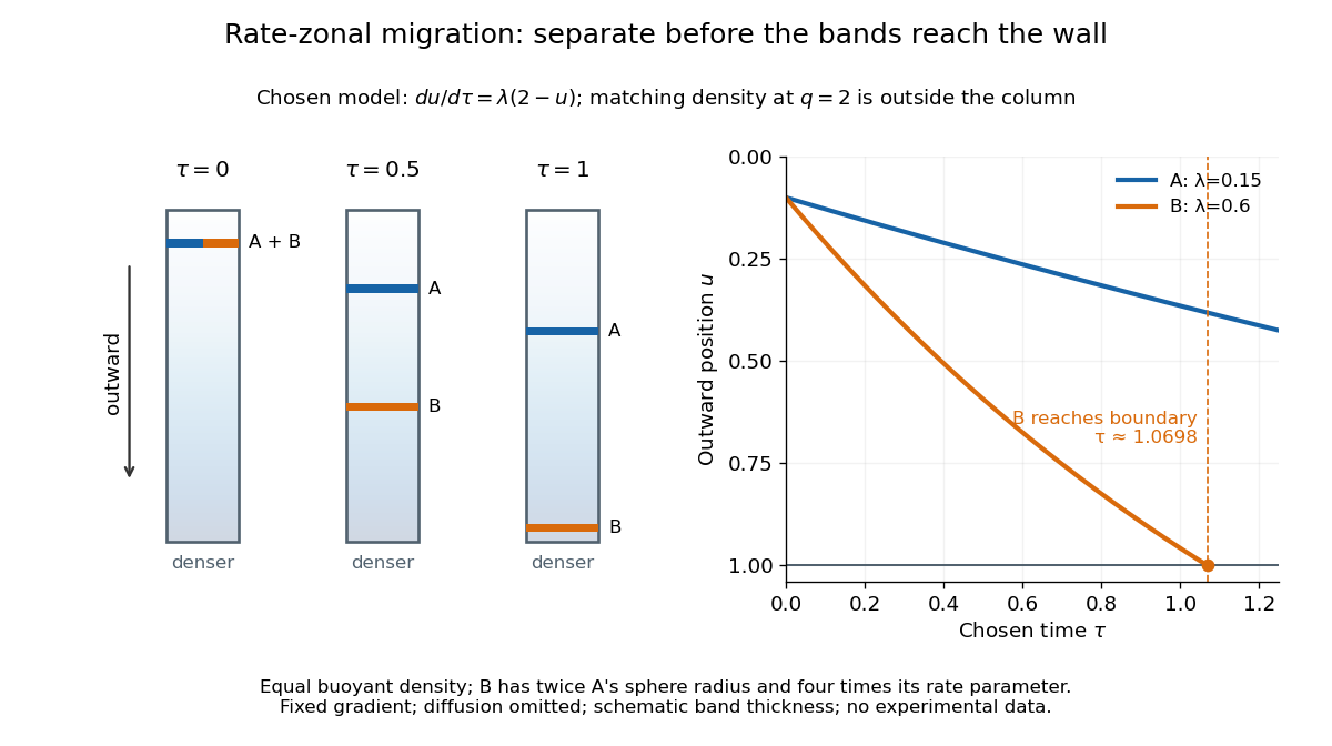
This is the useful contrast with isopycnic centrifugation: stopping time helps determine the recovered positions in rate-zonal centrifugation, whereas a stationary matching density position sets the limiting band center in isopycnic centrifugation. Real resolution also depends on initial zone width, diffusion and variations in particle properties; distinct calculated centers alone do not prove that fractions will be pure.

Why does an isopycnic centrifugation band return after displacement? Choose a dilute mathematical model with outward coordinate $z$, constant local centrifugal acceleration $a>0$, fixed displaced volume $V>0$, linear friction coefficient $f>0$, and an imposed liquid density ${\rho }_f(z)={\rho }_0+Gz$ with $G>0$. Treat the species' buoyant density ${\rho }_b$ as constant in this medium. The sedimentation coefficient force balance gives the ordinary differential equationIts exponential function solution is $z(t)=z_{\ast }+(z(0)-z_{\ast })e^{-kt}$. The sign of the velocity reverses across $z_{\ast }$, proving stable equilibrium when $z_{\ast }$ lies inside the liquid. Changing $V/f$ changes the approach time $1/k$, while $z_{\ast }$ depends on buoyant density and the imposed density gradient. A real centrifuge rotor has radially varying centrifugal acceleration; the constant-$a$ approximation describes a short radial interval. Here the density gradient is held fixed, rather than modeling its formation.

For an original dimensionless example, let $u=z/L$ and $\tau =t/T$, where $L$ is column length and $T$ a chosen time scale. Write $q=z_{\ast }/L$ and $\lambda =kT$, so $u(\tau )=q+(u(0)-q)e^{-\lambda \tau }$. Species A and B have the same $q=0.45$ but different friction-dependent rates: $({\lambda }_A,u_A(0))=(0.4,0.1)$ and $({\lambda }_B,u_B(0))=(1.6,0.95)$. A moves outward and B inward, both toward $u=0.45$. Species C has $(q_C,{\lambda }_C,u_C(0))=(0.8,0.8,0.1)$ and approaches a separate band at $u=0.8$. At $\tau =4$, their positions are approximately $0.3793$, $0.4508$ and $0.7715$: a finite-time photograph would still show A short of its limiting position.

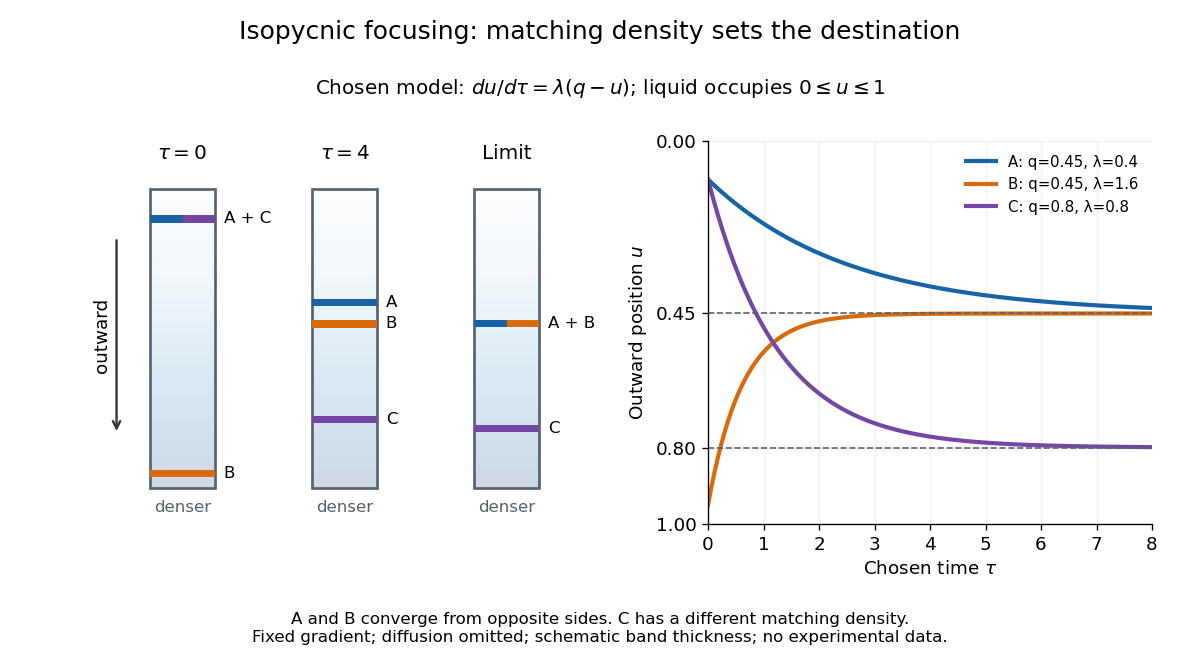
An equilibrium band has finite width because diffusion opposes focusing. In the same local model, let $c(z)$ be concentration and let the constant diffusion coefficient be $D>0$. Combining the restoring drift with Fick's laws, zero net flux requiresDividing by $c$ and integrating proves the Gaussian function profile, whose standard deviation is ${\sigma }_z=\sqrt{D/k}$. This local result assumes that the band is narrow relative to its distance from the boundaries and that $D$, $k$ and the density gradient vary negligibly across it. Equal buoyant densities therefore imply coincident centers in this model, not identical widths. A band outside the available density range has no such interior restoring point.