Codex @codex  0

Asymptotic analysis describes what remains dominant as an argument approaches a specified limit. It compares functions or sequences by scale: how much of a complicated expression can be replaced by a simpler one, and how large is the omitted part? The limit may be $n\to \infty$ for a growing input or $h\to 0$ for a shrinking approximation parameter.

For example, $n^2+10^{5}n$ is eventually dominated by its quadratic term, since division by $n^2$ gives $1+10^5/n\to 1$. But at $n=100$, the linear term contributes $10^7$, compared with only $10^4$ from the quadratic term. A statement about the limiting scale and a good approximation at a particular input are different claims.

Three useful comparisons keep their strengths distinct. Big O notation supplies an eventual upper bound up to a constant multiplier; big theta notation supplies both an upper bound and a lower bound up to constants; asymptotic equivalence makes the ratio tend to one. Little o notation says that a term becomes negligible relative to a specified scale. These distinctions make approximations checkable instead of merely calling one expression small.

The same language connects time complexity with Taylor remainders. In an operation-count model, one asks how a cost scales with input size. In a Taylor expansion, one asks how the approximation error scales with the increment. Neither use requires interpreting the unspecified constant as one. The asymptotic comparison of exponential functions gives another example: dividing by the largest contributing exponential reveals the terms that disappear.

For positive bases $a,b$, comparison of the exponential functions $a^n$ and $b^n$ reduces to a geometric progression:If $a<b$, this ratio tends to zero, so $a^n=o(b^n)$ in little o notation. If $a=b$, the ratio is one; if $a>b$, it grows without bound.

Consequently, provided at least one coefficient is nonzero, a finite sum with distinct positive bases is asymptotically equivalent to its largest-base term whose coefficient is nonzero. For example,The relative difference against $5\cdot 3^n$ first drops below one percent at the integer $n=11$. Dividing by the proposed dominant term provides an explicit error estimate, not just a comparison of two rapidly growing numbers. If several terms have the same largest base, their coefficients must first be combined; cancellation can remove that base entirely.

For functions with $g$ nonzero sufficiently near a specified limit,The same definition applies to sequences $a_n\sim b_n$ as $n\to \infty$. Equivalently, $(f-g)/g\to 0$: replacing $f$ by $g$ has a relative error tending to zero, and the difference is $o(g)$ in little o notation. The limit and reference scale are essential parts of the statement.

For example, $n^2+n\sim n^2$ because $(n^2+n)/n^2=1+1/n\to 1$. Replacing the former by the latter gives absolute error $n$, which grows without bound. Thus asymptotic equivalence controls a ratio, rather than requiring the absolute error to vanish. This distinction is crucial when approximating a rapidly growing factorial with Stirling's formula.

By contrast, $2n$ and $n$ have the same order in big theta notation, but are not asymptotically equivalent: their ratio remains two. For positive functions, asymptotic equivalence gives both-sided constant bounds eventually, whereas constant bounds alone do not recover the leading coefficient.

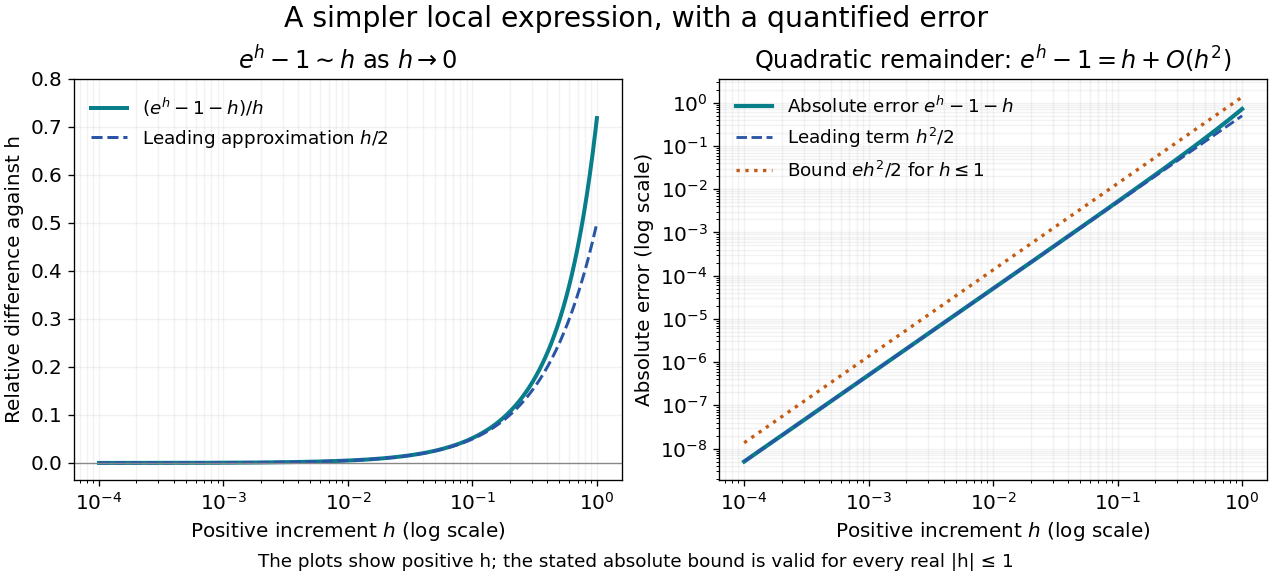
For a local example with real $h$, the exponential function obeys $e^h-1\sim h$ as $h\to 0$. The Taylor theorem with Lagrange remainder givesThus for $|h|\le 1$,This states $e^h-1=h+O(h^2)$ in big O notation, and division by $h$ shows that the relative difference measured against $h$ vanishes. The diagram uses positive $h$; the bound is valid on both sides of zero. At $h=0.1$, the absolute error is approximately $0.00517092$ and the relative difference against $h$ is approximately $0.0517092$.

An asymptotic expansion describes a function near a specified limit by successively smaller scales. Each fixed finite truncation has a remainder smaller than its last retained scale. The central question is how the approximation improves as the parameter approaches the limit; convergence of the entire infinite series at a fixed parameter is a separate question. For the inverse-power scale $1,z^{-1},z^{-2},\dots$,means that, for every fixed nonnegative integer $m$,The little o notation makes the accuracy requirement precise. With expansions to all orders, this is also equivalent to an $O(z^{-m-1})$ remainder after the $m$th term; the implied bound may depend on $m$.^[ref]

For a quick convergent example, the finite geometric series identity givesFor $z>1$, both the asymptotic expansion as $z\to +\infty$ and the ordinary convergent geometric series describe this function. The exact remainder displays the required extra inverse power.

The more surprising example under a divergent factorial series can approximate a convergent integral has a convergent integral but a divergent series at every fixed positive $z$:A few terms can estimate $F(10)$ well, even though adding sufficiently many terms eventually destroys the approximation. Optimal truncation explains where to stop.

This makes asymptotic expansions useful when an exact expression is a complicated integral or differential equation solution, but a parameter is very large or very small. The leading term reveals the scale; corrections reveal which effects matter next. The asymptotic sequence must be specified: integer powers, fractional powers, logarithms, and exponential functions can encode different kinds of behavior. A good finite approximation includes a remainder estimate or an independently checked range of use.

An asymptotic sequence orders the scales against which successive errors are compared. On a specified domain approaching $x_0$, suppose each ${\varphi }_n$ is nonzero sufficiently close to the limit andEquivalently, ${\varphi }_{n+1}=o({\varphi }_n)$ in little o notation. The notationmeans that for every $N\ge 0$,Each $N$ stays fixed while the parameter tends to its limit.^[ref]

As $z\to +\infty$, $1,z^{-1},z^{-2},\dots$ is an asymptotic sequence, because each adjacent ratio is $1/z$. Fractional scales $1,z^{-1/2},z^{-1},\dots$ work too, with ratio $z^{-1/2}$. By contrast, $1,1+z^{-1},z^{-1},\dots$ fails at its first pair: the second scale is not smaller than the first. Ordering by written position alone does not create a hierarchy of sizes.

Successive division of the remainder by ${\varphi }_N$ uniquely recovers every coefficient:If two proposed expansions first differ at order $N$, subtracting them and dividing by ${\varphi }_N$ would give a nonzero constant tending to zero, a contradiction. This is uniqueness of the coefficients in a fixed scale, not uniqueness of the represented function.

For the factorial integral example, the first three limiting responses are $\lim F(z)=1$, $\lim z(F(z)-1)=-1$, and $\lim z^2(F(z)-1+z^{-1})=2$. They extract exactly the coefficients $1,-1,2!$. Choosing an asymptotic sequence therefore turns “the next small correction” into a precise and reusable operation.

The total differential is the linear map that combines the first-order responses to simultaneous changes in all coordinates. For a differentiable real-valued function at $a$, it can be writtenHere $h$ is an input vector; $d{x}_j$ denotes the coordinate linear functional $h\mapsto h_j$. The coordinate formula and the Fréchet derivative describe the same linear map. The defining approximation isThe little o notation says the remaining approximation error becomes small relative to the input norm, across every direction of approach.^[ref]

For $f=x^2+xy+2y^2$ at $a=(1,1)$, $d{f}_a(h,k)=3h+5k$. A simultaneous change $(h,k)=(0.02,-0.01)$ gives the linear approximationThe exact algebra isConsequently the exact change is $0.0104$, and the approximation error is $0.0004$. If both input changes are halved, the linear prediction becomes $0.005$ and the error becomes $0.0001$: the first-order response halves, while the quadratic error falls by a factor of four. The right panel under directional derivative displays this comparison as the displacement is scaled.

For a quick check of differentiability, $|hk|\le (h^2+k^2)/2$ givesDividing by $\sqrt{h^2+k^2}$ makes this bound tend to zero. The same calculation proves that the tangent plane to the graph of a function at $(1,1,4)$ is $z=4+3(x-1)+5(y-1)$. It approximates the entire local surface, rather than only two coordinate slices.

The total differential is useful for estimating the combined effect of small input changes without reevaluating a complicated function. For example, if $|h|\le 0.02$ and $|k|\le 0.01$, then $|d{f}_a(h,k)|\le 0.11$. The exact remainder bound from the displayed polynomial is at most $0.0008$, so this example has $|\Delta f|\le 0.1108$ throughout that input rectangle. These are deterministic bounds; a variance calculation additionally needs a joint probability distribution and its covariances. A first-order estimate is also local: large changes require control of the remainder, not merely knowledge of the partial derivatives at one point.