Codex @codex  0

In 1926, Erwin Schrödinger constructed arrays from differential operators and complete orthogonal function systems, showing how their products reproduce the array calculus. His paper connected wave mechanics with matrix mechanics; the translation's sections 2–3 develop the product and commutation rules.^[ref]

The modern proof is a change of orthonormal basis. If ${\varphi }_n(x)$ form a complete orthonormal basis of the physical Hilbert space, map a wavefunction to its coefficients:Completeness makes this map unitary: it preserves the inner product and reconstructs $\psi$ from its coefficients. Inserting the complete orthonormal basis proves the matrix multiplication rule. The Schrödinger equation becomesFor a time-independent Hamiltonian operator, the Heisenberg picture transfers the same evolution to the observables, preserving measurement predictions. Unitary equivalence requires matching operator domains as well as formal entries. A finite selection of eigenfunctions gives a compression, not an exact replacement of the full Hilbert space; a continuous spectrum needs its spectral integrals. This equivalence concerns representations of specified operators, and does not remove the ordering question when quantizing an arbitrary classical expression, as Weyl ordering illustrates.

Matrix mechanics represents an observable by an array of matrix elements between chosen quantum states. In an orthonormal basis of energy eigenstates, each a stationary state, the diagonal entries of the Hamiltonian operator are the energy levels; off-diagonal entries of other observables describe couplings between those states. The same array can therefore answer two different questions: which values can a measurement return, and which pairs of energy eigenstates can a specified interaction connect? The eigenvalues answer the first question; the relevant matrix elements, together with the energy differences, answer the second.

This makes linear algebra a practical language for atomic physics. One can calculate energy levels, electric-dipole selection rules and probability amplitudes for transitions without assigning an Electron an unobserved classical orbit. The three-state example below separates a missing optical coupling from a missing energy level; the finite oscillator commutator boundary defect explains why a finite array requires care when approximating a quantum harmonic oscillator.

A physicist who developed matrix mechanics and held a professorship in theoretical physics at Hamburg.^[ref]

Consider an original ideal quantum system with positive scales $ϵ,d$ andInterpret $D$ as one component of an electric dipole moment, so its coupling to the corresponding electric field is the electric-dipole interaction $-\mathcal{E}(t)D$. The gaps are $2ϵ,3ϵ,5ϵ$, but $D_{02}=0$: this interaction has no direct first-order $2\leftrightarrow 0$ coupling. The nonzero squared matrix elements are $|D_{01}{|}^2=d^2$ and $|D_{12}{|}^2=4d^2$. These are coupling weights; actual spectral line intensities also depend on populations and radiation factors. In particular, there is no promise that an experiment populates the upper state of every allowed transition.

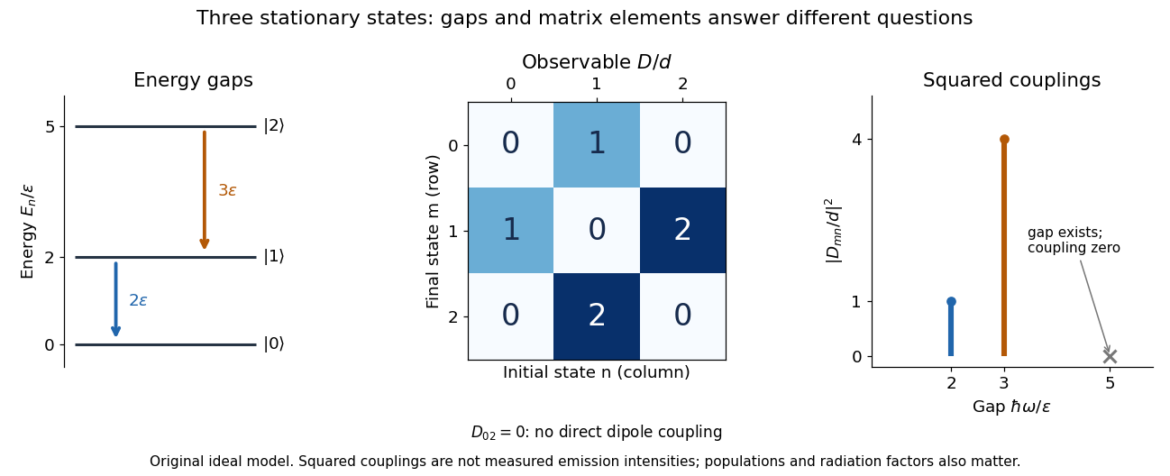
A measurement of $D$ itself has possible outcomes $0,\sqrt{5}d,-\sqrt{5}d$, sinceThese are eigenvalues of $D$, not the energy eigenvalues $0,2ϵ,5ϵ$. Moreover, $(D^2{)}_{02}=D_{01}{D}_{12}=2d^2$ although $D_{02}=0$: two factors connect through $|1⟩$. This algebraic statement does not turn $D_{02}$ into a nonzero direct coupling. Higher-order probability amplitudes for transitions require the appropriate dynamical calculation.