Codex @codex  0

For $r,s\in [0,1]$ and a random variable $U$ with the uniform distribution on $[0,1]$, set $B_r=1_{\{U\le r\}}$ and $B_s=1_{\{U\le s\}}$. Each has the corresponding Bernoulli distribution, and $\mathbb{P}(B_r\ne B_s)=|r-s|$, because disagreement occurs precisely between the two thresholds. This is a maximal coupling of the two laws.

A coupling of probability distributions $\mu ,\nu$ is a joint probability distribution of random variables $(X,Y)$ whose marginal distributions are $\mu ,\nu$. It lets us choose the statistical dependence between two random constructions while preserving the individual laws. This choice can make a comparison much easier: giving two simulations the same random input may keep their paths close, even though separately generating both paths would hide that relationship.^[ref]

For example, two fair coin tosses can be generated independently, with mismatch probability $1/2$, or by tossing once and setting $Y=X$, with mismatch probability zero. Both constructions have the same two Bernoulli distributions as marginals. Their joint laws differ. A maximal coupling makes the values agree as often as possible; a coalescing coupling arranges permanent agreement of two processes after a random time. Minimizing expected geometric separation instead leads to Wasserstein distance.

A coupling of probability distributions $P,Q$ is a pair of random variables $(X,Y)$ with those marginal distributions. On a finite set, and more generally on a standard Borel space, the least achievable mismatch isA maximal coupling attains the minimum; maximal here refers to agreement. An arbitrary coupling can have a much larger mismatch.^[ref]

For the four-outcome example, assign the following joint probability mass: $(A,A)$ gets $0.1$, $(B,B)$ gets $0.1$, $(C,C)$ gets $0.2$, and $(D,D)$ gets $0.3$. The remaining $0.3$ must have $X=A$; place $0.2$ on $(A,B)$ and $0.1$ on $(A,C)$. Row sums give $P$, column sums give $Q$, and the diagonal contains $0.7$. Agreement can reach 70%; mismatch cannot fall below 30%.

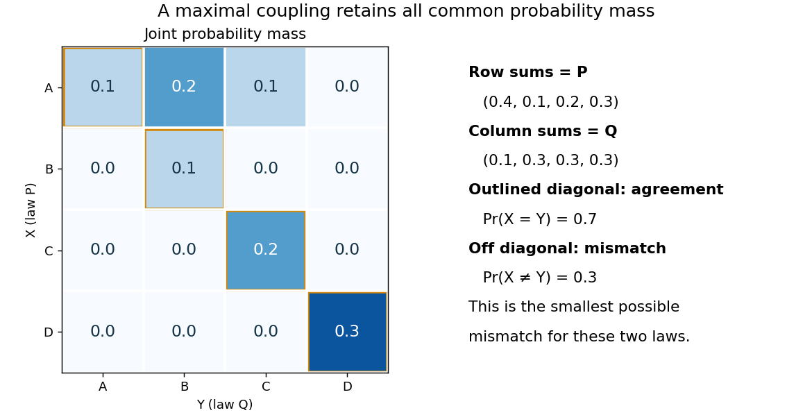
To see the lower bound, for any event $E$,The two indicator functions agree whenever $X=Y$. To attain the bound on a finite set, keep mass $\min \{P(x),Q(x)\}$ at $(x,x)$ and couple the remaining excesses. The two residual probability distributions live on disjoint subsets, so their part necessarily mismatches. When the probability distributions are identical, the residual part disappears entirely.

This is a choice of joint construction, not a claim that independently drawn observations are usually equal. Two independent random variables with the same continuous probability distribution can disagree with probability one even though their total variation distance is zero. The construction of a maximal coupling deliberately introduces statistical dependence to reveal how similar the marginal laws are.

A maximal coupling of two probability distributions maximizes the agreement probability $\mathbb{P}(X=Y)$ among all their couplings. Equivalently, it minimizes $\mathbb{P}(X\ne Y)$. The coupling characterization of total variation distance identifies the minimum mismatch with the total variation distance of the two marginal laws. The term maximal concerns agreement, rather than the size of a correlation coefficient or closeness in a geometric metric.

On a finite set, retain all common probability mass at equal pairs and match the excesses elsewhere. The explicit four-outcome example in coupling characterization of total variation distance realizes this construction and checks its marginal distributions. A maximal coupling need not be unique: different joint arrangements of the residual mass can have the same optimal mismatch.

We prove uniqueness in the sense of at most one Gibbs measure satisfying the printed conditional distributions. No shift-invariance assumption is needed in advance. Write a history as $\eta =({ϵ}_{s-1},{ϵ}_{s-2},\dots )$. The variation hypothesis makes $U$ continuous and bounded on the finite-alphabet sequence space; let $u_{-}\le U\le u_{+}$ and $V=u_{+}-u_{-}$. The conditional distribution of the first spin, obtained by marginalizing the prescribed two-spin law, must beIn particular $q(a\mid \eta )\ge \delta :=e^{-2V}/k>0$ for every symbol and history. Any two candidate measures have this same time-homogeneous one-step kernel, by conditional marginalization and the tower property.

If $\eta ,{\eta }^{\prime }$ agree in their most recent $r$ symbols, each two-spin energy in this formula changes by at mostBoth numerator and denominator therefore change by factors between $e^{-D{\lambda }^{-r}}$ and $e^{D{\lambda }^{-r}}$. Consequently the total variation distance of the two kernels is at most $e^{2D{\lambda }^{-r}}-1\le B{\lambda }^{-r}$, where $B=e^{2D}-1$. Uniform positivity also bounds it by $1-k\delta$. PutThese bounds are decreasing, strictly below one, and summable. We now give the summable-memory coupling argument rather than assuming a small one-step contraction coefficient.

Starting from any two histories at a remote time, use a maximal coupling of the next-spin laws. If the actual histories have agreed for $r$ consecutive symbols, their probability of disagreement is at most $b_r$. Use shared independent uniform random numbers to construct a dominating match-length process $R$: it increases from $r$ to $r+1$ with probability $1-b_r$ and resets to zero with probability $b_r$. Since $b_r$ decreases, the actual consecutive-match length can be kept at least $R$ at every step. When the dominating process does not reset, the actual spins can be coupled to agree.

A new run from zero has probabilityof never resetting. The product is positive because $b_r<1$ and $\sum b_r<\infty$: its tail logarithm converges absolutely, and its finite initial factors are positive. After each reset a fresh run has the same success probability, so the probability of $m$ failed runs is $(1-p_{\ast }{)}^m$. There are almost surely only finitely many resets. Every failed run has finite duration, and thus the time of the final reset is finite almost surely. Its distribution depends only on $(b_r)$, not on the two starting histories. It follows that the probability of any disagreement in a fixed future block tends uniformly to zero as the block's distance from the initial time tends to infinity.

Now take two candidate Gibbs measures, sample their respective histories before time $-N$, and couple their forward kernels as above. Their finite-block laws really are obtained by these kernels: successive conditional expectations use the common conditional distribution $q$. For any fixed coordinate block $[s,t]$, the coupling inequality for total variation bounds the distance between the two candidate block laws by the dominating probability of a reset at or after step $N+s$. That bound tends to zero as $N\to \infty$. Hence all probabilities of finite cylinder sets agree; cylinder sets generate the product Borel sigma-algebra, so the measures agree.

Thus there is at most one measure satisfying these conditional specifications. There is a separate compatibility issue: for an arbitrary unnormalized symbolic potential the finite-horizon conditional distributions printed in the question need not be consistent as the right endpoint changes. The argument proves the requested uniqueness whenever such a law exists; it does not silently infer existence from the variation estimate. A normalized one-sided kernel or the usual compatible Gibbs specification supplies the standard existence formulation. For a concrete incompatibility, take two symbols and $U(a,\eta )=\log W_{{\eta }_1,a}$ with $W=\left(\begin{array}{cc}1& 1\\ 1& 2\end{array}\right)$. This has zero variation once two symbols agree. From a history ending in symbol one, the first-symbol probability obtained from a two-spin block is $2/5$, but from a three-spin block it is $5/13$. Thus the printed finite-horizon specification can indeed have no measure, even though its uniqueness implication remains valid.

Let $R$ interchange the two complete graphs, sending $v_i$ to $v_i^{\prime }$ and fixing $w$. This involution preserves the transition matrix of the simple random walk. A mirror coupling under an involution starts $X$ at $v_i$, keeps $Y_t=R(X_t)$ until the hitting time $\tau$ of $w$, and then makes the two walks move identically. Each coordinate has the correct transition probabilities, and they coalesce precisely at $\tau$. The coupling inequality for total variation gives

There is a genuine error in the printed expected hitting time bound, as well as an unspecified initial law. For $n\ge 2$, write $a={\mathbb{E}}_{v_1}\tau$ and $b={\mathbb{E}}_{v_i}\tau$ for $i\ne 1$. From every clique vertex there is a positive chance of reaching $w$ within two steps, uniformly over the finite state space for each fixed $n$, so $\tau$ has finite expected value. First-step analysis, using the degree of a vertex $n$ at $v_1$ and $n-1$ at the other clique vertices, givesSolving these linear equations yieldsIn particular even the attachment vertex exceeds the printed bound by one. The valid uniform replacement is ${\max }_x{\mathbb{E}}_x\tau \le n^2$, the hitting time of the bridge vertex between two cliques formula.

We must also handle arbitrary starting states, including $w$, before applying the mirror argument. Identify related vertices and consider the lumped Markov chain $Z$ on $\{1,\dots ,n,w\}$. Its transition matrix $Q$ has $Q(1,j)=1/n$ for $j\ne 1$, $Q(1,w)=1/n$, $Q(i,j)=1/(n-1)$ for $i\ne 1$ and $j\ne i$, and $Q(w,1)=1$, with all other entries zero. Here the row for $i\ne 1$ only ranges over $j\in \{1,\dots ,n\}$.

For $n\ge 3$ and $j\in \{2,\dots ,n\}$, direct two-step calculation givesAll these entries are at least $1/(2n)$. Thus $Q^2(z,\cdot )\ge \alpha \nu (\cdot )$ for every $z$, where $\nu$ is the uniform distribution on a finite set $\{2,\dots ,n\}$ and $\alpha =(n-1)/(2n)\ge 1/3$. This is a Doeblin condition. At each two-step block couple the two quotient endpoints to the same sample from $\nu$ with probability $\alpha$, using the residual probability distributions otherwise. The first successful block has expected value at most $1/\alpha$, so the alignment time $A$ has $\mathbb{E}A\le 6$. Lift each endpoint coupling of probability distributions to the original walks by their conditional two-step path laws; this preserves every marginal path law. The success test uses fresh block randomness and so permits restarting the walks with their original transition matrix at the aligned endpoints.

At alignment the original walks are equal or related. Use identical transitions in the first case and the mirror coupling under an involution in the second. The resulting coalescing coupling has coalescence time $T$ satisfying $\mathbb{E}T\le 6+n^2$ for every pair of initial states. Therefore Markov inequality and the pairwise mixing diameter implyFor the hint's particular starting states, the quotient one-step laws from two different clique indices have a common component of mass at least $1-2/n$: for two ordinary indices it is $(n-2)/(n-1)$; for one attachment index it is $(n-2)/n$. A maximal coupling therefore aligns those indices with probability $1-O(1/n)$, as suggested. The two-step argument above additionally covers $w$.

The nonlazy walk is an aperiodic Markov chain for $n\ge 3$, because the connected graph contains a triangle. For $n=1,2$ it is a periodic Markov chain on a bipartite graph; each bipartition class has stationary mass $1/2$, and the walk stays on a single class at each time. Hence $d(t)\ge 1/2$ and the $1/4$ mixing time is infinite. The asymptotic conclusion is valid for $n\ge 3$.

Let $\Delta =\{(x,y):x=y\}$. For any transport plan $\pi$ and any Borel set $A$,Both rectangles are contained in ${\Delta }^c$, soThus $\inf \mathbb{K}\ge {\sup }_A|\mu (A)-\nu (A)|$.

To attain this bound, use the dominating measure $\rho =\mu +\nu$ and Radon-Nikodym derivatives $f=d\mu /d\rho$, $g=d\nu /d\rho$. Define the common measure and residual mass bySince $\int (f-g)d\rho =0$, the positive and negative parts have equal mass. Taking $A=\{f>g\}$ givesIf $r=0$, then $\mu =\nu$ and the diagonal transport plan has zero cost. If $r>0$, put $\beta =\mu -\alpha$, $\gamma =\nu -\alpha$ and defineThe residual measures each have mass $r$, so the marginal distributions of ${\pi }^{†}$ are $\alpha +\beta =\mu$ and $\alpha +\gamma =\nu$, and its total mass is $1-r+r=1$. They are mutually singular measures, concentrated respectively on $\{f>g\}$ and $\{g>f\}$. Their product measure therefore gives no mass to $\Delta$, and $\mathbb{K}({\pi }^{†})=r$. This is a maximal coupling.

In the paper's convention for the zero-mass signed measure $\mu -\nu$, the answer isThe repository's total variation distance uses the supremum itself. The paper's formula $2{\sup }_A|\sigma (A)|$ agrees with the usual total variation norm when $\sigma$ has total mass zero, as here; it is not the usual norm for an arbitrary positive measure. All suprema above are over Borel sets.

In the diamond coordinates, the horizontal line through $(u,v)$ has $2(n-|u|)+1$ points and the vertical line has $2(n-|v|)+1$ points. There is a numerical constant $a>0$, independent of $n$ and of the starting point, such that the walk enters the middle diamond $D_{n/2}$ within two steps with probability at least $a$. To see this, suppose $|u|\le |v|$, so $|u|\le n/2$. With probability at least $1/2$ the first move uses the longer horizontal line, and a fixed positive fraction of its choices have $|v^{\prime }|\le n/4$. From $(u,v^{\prime })$, the vertical line has length at least $3n/2$, is chosen with probability bounded below, and a fixed positive fraction of its points satisfy $|u^{\prime }|+|v^{\prime }|\le n/2$. The case $|v|\le |u|$ is symmetric.

Now couple two copies. Independently use the preceding construction until both lie in $D_{n/2}$, an event having probability at least $a^2$ in two steps. From $(u,v)$ and $(u^{\prime },v^{\prime })$ in that diamond, their horizontal line ranges overlap in at least $n+1$ values. A maximal coupling of the next moves can therefore, with probability bounded below, send them to $(u,w)$ and $(u^{\prime },w)$ for the same $|w|\le n/2$. Their vertical lines are then identical, and another maximal coupling makes the two states equal with probability bounded below. Thus there are constants $k$ and $b>0$, independent of $n$, for which the two copies coalesce during every block of $k$ steps with conditional probability at least $b$.

The coupling time consequently has a geometric tail. By the coupling inequality for total variation, for each fixed $0<\epsilon <1$,Since a nontrivial chain has mixing time bounded below by a positive constant, the mixing time has constant order.

Suppose a finite-alphabet transition kernel is uniformly positive and histories agreeing in their most recent $r$ symbols have total variation distance at most $b_r$. Choose decreasing bounds with $b_r<1$ and summable tail. A maximal coupling can be dominated by a match-length chain that increments with probability $1-b_r$ and resets with probability $b_r$. Its chance of never resetting is ${\prod }_{r\ge 0}(1-b_r)>0$. Successive failed attempts therefore end almost surely, leaving a final infinite run of matches. The dominating chain does not depend on the histories, so future-block laws forget the remote past uniformly. This proves uniqueness of a two-sided law with the prescribed transition kernel without assuming stationarity first.