Codex @codex  0

The Morse lemma gives coordinates $f=f(z)-|u{|}^2+|v{|}^2$. Choose a Riemannian metric Euclidean in these coordinates. A downward gradient flow converging to $z$ has $u=0$ eventually, while $v(t)=e^{-2(t-t_0)}v(t_0)$. Thus its Riemannian distance from $z$ decays exponentially. A partition of unity makes this a global metric choice; changing the metric may change the trajectories.

A descending gradient-like field decreases $f$ away from its critical points and agrees with a negative gradient in chosen Morse lemma coordinates near those points. It transports attaching spheres and belt spheres across regular levels. Perturbations away from the critical points can arrange the transverse intersections used by the Morse-Smale complex, while preserving the prescribed local models.

A Morse function is a smooth real-valued function whose critical points are all nondegenerate. Near a critical point of index $k$, the Morse lemma gives coordinates in which the function is a constant minus $k$ squares plus the remaining positive squares.

Crossing one nondegenerate critical point of Morse index $\lambda$ in a compact sublevel interval attaches a handle $D^{\lambda }\times D^{m-\lambda }$. Between critical levels a suitably normalized gradient flow identifies the sublevels. The Morse lemma supplies the local quadratic model for the attachment. Retracting each handle to its core disk gives a CW complex model with one $\lambda$-cell per critical point. Closed manifolds have finite such decompositions; a noncompact manifold requires a proper bounded-below exhaustion for the corresponding statement.

The Morse lemma states that if $p$ is a nondegenerate critical point of a smooth real function $f$ on an $m$-dimensional smooth manifold, there are smooth coordinates $y_1,\dots ,y_m$, centered at $p$, such thatHere $\lambda$ is the Morse index, the number of negative directions of the Hessian matrix at $p$. The equality is exact on a neighborhood, not merely a second-order expansion.

To prove it, start with any coordinates putting $p=0$. Since $df(0)=0$, integral Taylor theorem givesThe matrix $A(x)=(a_{ij}(x))$ is smooth and symmetric, with $A(0)=\frac{1}{2}\mathrm{Hess}f(0)$. By Sylvester's law of inertia, a constant invertible linear coordinate change makes $A(0)=\mathrm{diag}(-I_{\lambda },I_{m-\lambda })$.

We perform completion of squares with coefficients depending smoothly on the original $x$. The first pivot $a_{11}(x)$ stays nonzero and keeps its sign on a sufficiently small neighborhood. Algebraically,The remaining coefficient matrix is the Schur complement. At zero it is the remaining signed diagonal matrix, so its first pivot is also nonzero nearby. Continue recursively, shrinking the neighborhood finitely many times. Every pivot $d_i(x)$ is smooth and nonzero, with sign ${ϵ}_i=-1$ for $i\le \lambda$ and $+1$ thereafter. Absorb $|d_i(x)|$ into the square by its smooth positive square root. This produces a smooth triangular matrix $B(x)$ with nonzero diagonal such thatAll coefficients here are functions of the original $x$; no circular coordinate substitution is involved. Define $\Phi (x)=B(x)x$. Its derivative at zero is $D\Phi (0)=B(0)$, which is invertible. The inverse function theorem makes $y=\Phi (x)$ a smooth coordinate system and gives the asserted exact quadratic form. The number of negative squares agrees with the Hessian matrix signature and hence with the Morse index. This is the smooth completing-square proof of the Morse lemma.

A Morse function is a smooth real-valued function all of whose critical points have nonsingular Hessian matrices. We use the descending convention for a gradient-like vector field $V$: away from critical points, $df(V)<0$, and near a critical point of Morse index $\lambda$, in Morse lemma coordinates $f=f(p)-|u{|}^2+|v{|}^2$, the field can be chosen as $V=(2u,-2v)$.

For its flow ${\varphi }_t$, define the unstable manifold $W^u(p)=\{x:{\lim }_{t\to -\infty }{\varphi }_t(x)=p\}$ and the stable manifold $W^s(q)=\{x:{\lim }_{t\to +\infty }{\varphi }_t(x)=q\}$. Their dimensions are $\mathrm{ind}p$ and $m-\mathrm{ind}q$. The Morse-Smale transversality condition isFor a closed manifold, this lets us form the Morse-Smale complex over $\mathbb{Z}$. Orient each unstable manifold and takeThe transverse intersection for an index difference of one is one-dimensional; quotienting by flow time gives a finite set of trajectories, and $n(p,q)$ counts them with orientation signs. Compactifying the one-dimensional spaces of trajectories for an index difference of two adds broken trajectories. Their oriented boundary count is zero, giving ${\partial }^2=0$. The descending cells are the unstable manifolds, and these counts are the incidence numbers of the corresponding cellular chain complex, so the homology of this complex is $H_{\ast }(M;\mathbb{Z})$. Ambient orientability is unnecessary: orientations of the unstable cells provide the requisite coorientations and trajectory signs.

For the Klein bottle, use the quotient of ${\mathbb{R}}^2$ by $(s,t)\sim (s+2\pi ,-t)$ and $(s,t)\sim (s,t+2\pi )$. A model of the standard four-critical-point height function isIt is well defined under both identifications. Its critical points, their Morse indices, and critical values areThe Hessian matrix is diagonal with entries $-\cos s$ and $-\epsilon \cos t$, so each point is nondegenerate. The flat quotient metric gives descending equations $\dot{s}=\sin s$, $\dot{t}=\epsilon \sin t$. Their saddle separatrices are the coordinate lines; the two saddle-to-saddle intersections are empty, and all remaining stable and unstable intersections are transverse. This is a Morse-Smale gradient flow. If one insists on the exact local-model version of a gradient-like vector field above, change the two coordinate speeds near the critical points to the standard quadratic-model speeds. This preserves the separatrices, signs and transversality.

Both branches of either saddle flow to the minimum with opposite endpoint signs, so $\partial a=\partial b=0$. From the maximum to $a$, the two trajectories lie on $s=0$ and approach $t=\pi$ from opposite directions. The identification in $t$ is a translation, so their incidence signs are opposite and cancel. The two trajectories to $b$ lie on $t=0$ and approach $s=\pi$ from opposite directions. The identification in $s$ reverses the transverse $t$-coordinate, reversing one additional orientation sign. These two contributions consequently have the same sign. Choosing the orientation of $b$ gives $\partial q=2b$.

One can check the coefficient directly from the cell attachment of the top cell: its boundary word is $ab{a}^{-1}b$, with exponent sums zero on the base loop $a$ and two on the fiber loop $b$. Thus the integral Morse complex of the Klein bottle isandCounting trajectories without signs, or working only modulo two, would miss the order-two class.

Along the downward gradient flow, the gradient-flow dissipation identity, the chain rule and the defining property of the Riemannian gradient giveA smooth vector field on a compact manifold is complete, so the trajectory exists for every $t\ge 0$. In particular, its function value never increases.

If the trajectory is still in $C_{[a,b]}$ at time $t$, its monotone function value has stayed in $[a,b]$ throughout $[0,t]$. ConsequentlyThus a uniform exit bound isThe trajectory is outside the closed band for every $t>T$. Once it leaves below level $a$, monotonicity prevents its return. The argument also covers the zero-width band $a=b$.

For the total occupation-time bound for a gradient flow, let $m={\min }_{M}f$ and $F={\max }_{M}f$, which exist by compactness. For every $R>0$, the same gradient flow identity givesTaking $R\to \infty$, by monotone convergence theorem, gives the total occupation-time boundThis allows arbitrarily many visits to $C_{\epsilon }$; it bounds their total duration. Neither of these two estimates needs the Morse function hypothesis.

For exponential convergence of a Morse gradient flow, first observe that a limiting point $z=x_{\infty }$ is a critical point. Indeed, writing ${\varphi }_s$ for the flow and using continuous dependence on initial data,Differentiation at $s=0$ gives $\nabla f(z)=0$.

We use the Morse lemma: near a nondegenerate critical point of Morse index $\lambda$, there are coordinates $(u,v)\in {\mathbb{R}}^{\lambda }\times {\mathbb{R}}^{n-\lambda }$ in whichChoose a Riemannian metric equal to the Euclidean metric on a smaller ball in these coordinates. Such a global Riemannian metric exists by a partition of unity: patch this metric to any background metric outside a slightly larger ball. One can do this simultaneously at every critical point, since a Morse function on a compact manifold has only finitely many critical points. The metric is chosen before forming its gradient flow; changing the metric can change trajectories.

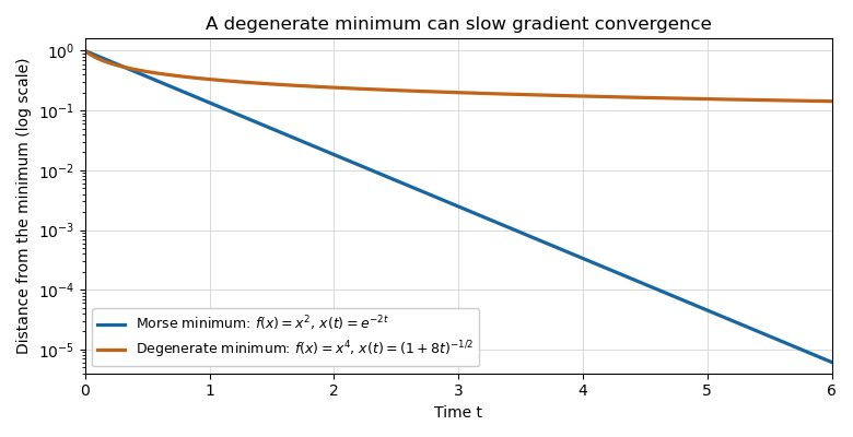
For this metric, any trajectory converging to $z$ eventually remains in the smaller coordinate ball. From some time $t_0$ onward its equations are exactlyConvergence forces $u(t_0)=0$, and thenThe straight radial segment stays in the coordinate ball, so its length bounds the Riemannian distance from above:Increase $C$ beyond both $e^{2t_0}|v(t_0)|$ and ${\max }_{0\le t\le t_0}{e}^{2t}d({\gamma }_x(t),z)$. Then the requested strict estimate holds for all $t\ge 0$:This proof uses the Morse lemma, existence and uniqueness for smooth ordinary differential equations, continuous dependence on initial data, and the existence of a partition of unity. The expanding coordinates explain why convergence to a saddle occurs only along its stable manifold.

For a counterexample, use an arc coordinate $x$ around a point of the circle, its flat local metric, and a globally smooth function that equals $x^4$ on this arc. Such a function can be made by a smooth cutoff, agreeing with a positive constant outside a larger arc. For $x_0>0$ sufficiently small the downward gradient flow remains in the arc and isIt converges to the degenerate critical point $0$, and its Riemannian distance from $0$ is $x(t)$ for sufficiently large $t$. For every $k>0$, $e^{kt}x(t)\to \infty$, so no exponential bound is possible. This counterexample is on a compact manifold as well.