Codex @codex  0

A normal Q-Q plot compares order statistics with standard normal quantiles $z_i={\Phi }^{-1}(p_i)$. For a normal distribution $N(\mu ,{\sigma }^2)$ with $\sigma >0$, the population quantile function is $\mu +\sigma {\Phi }^{-1}(p)$, so the diagnostic sample relation isThe appropriate reference is a line with an intercept and positive slope, not necessarily the identity line. A line can be fitted through two central sample quantiles; R's qqline uses the quantile levels $p=0.25$ and $p=0.75$ by default. Neither that line nor its fitting rule is part of the definition of a normal Q-Q plot. ^[ref]

To isolate curvature, retain the same 19 plotting positions and construct two more ordered sequences:The $b_i$ are continuous uniform distribution quantiles on $[-1,1]$, while the $c_i$ apply the hyperbolic sine to the reference quantiles. Both examples are symmetric about zero. At ranks $1,10,19$, $b_i$ is approximately $-0.947368,0,0.947368$ and $c_i$ is approximately $-1.812618,0,1.812618$. Again, these are constructed values rather than random draws or real data.

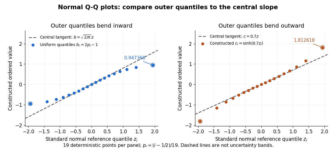
Read these shapes relative to their central slope. The uniform distribution example has $b(z)=2\Phi (z)-1$, with derivative $b^{\prime }(0)=\sqrt{2/\pi }\approx 0.797885$; at the upper endpoint the tangent predicts $1.546246$, while $b_{19}=0.947368$. Its lower end lies above the tangent and its upper end below it: the outer quantiles are compressed. The hyperbolic sine example has $c^{\prime }(0)=0.7$; its tangent predicts $1.356552$ at the upper endpoint, while $c_{19}=1.812618$. Its lower end lies below the tangent and its upper end above it: the outer quantiles are stretched. Unequal departures at the two ends can suggest skewness. The direction of these descriptions assumes that reference quantiles are horizontal and observed values vertical. The graphs illustrate finite-range shape differences; a sample pattern cannot establish an asymptotic tail probability law or membership in a heavy-tailed distribution class.

A nearly straight normal Q-Q plot is a diagnostic, not a proof of a normal distribution or a formal hypothesis test. Random statistical samples fluctuate, particularly at extreme order statistics, and apparent curvature depends on sample size, plotting positions and the reference line. A calibrated hypothesis test or uncertainty band requires its own assumptions and must account for parameters estimated from the same observations. Sorting also discards the original observation order: rearranging a time series leaves its Q-Q plot unchanged, so the plot cannot establish independence.

For a normal linear model, R's diagnostic normal Q-Q plot uses standardized regression residuals, also called internally studentized residuals. ^[ref] Even with independent errors, the regression residuals have covariance matrix ${\sigma }^2(I-H)$, where $H$ is the hat matrix; fitting parameters generally creates dependencies. Dividing by a shared estimated standard deviation creates further dependence, and the distribution of an internally studentized Gaussian residual is not exactly the standard normal distribution. The normal Q-Q plot therefore helps assess error shape alongside other diagnostics rather than certifying independent normal random variables.

The missing output is needed to identify the actual regression formula, response column, transformations and coefficient estimates. A useful possible analysis regresses the maintained-school percentage among acceptances on the corresponding percentage among applications, allowing for year; it must be described as a model of college-level composition, not a direct estimate of individual acceptance probabilities.

For instance, if $a_{jt}$ and $p_{jt}$ are these two percentages, a normal linear model might specify $\mathbb{E}(a_{jt})=\alpha +\beta p_{jt}+\delta 1_{\{t=2000\}}$, with a slope-by-year interaction term if needed. The intercept is the expected response at zero predictor, often an extrapolation; the slope is a percentage-point change in acceptance composition per percentage-point change in application composition. A slope of one is not by itself evidence of equal acceptance chances: equal chances within every college would give the entire relation $a_{jt}=p_{jt}$, including zero intercept and no year shift. A fit with positive slope mainly confirms that applicant composition helps predict acceptance composition.

Regression diagnostics should include residuals versus fitted values and predictors, a residual normal Q-Q plot, checks of heteroscedasticity, regression leverage, studentized residuals and Cook's distance. The aggregate mature-college category merits an influence check and a sensitivity analysis: combining several colleges can conceal different within-college patterns. Repeated observations from the same college across years may have correlated errors, so treating them as independent needs justification. Check nonlinearity, the year interaction and the effects of excluding no observation except with a substantive reason.

Percentages are bounded, and their precision depends on their denominators. A simple weighted least squares or binomial analysis requires the underlying numbers accepted, not merely percentages. For a proportion based on $m$ people, the working variance is $\pi (1-\pi )/m$ under independent sampling, rather than constant across colleges. If the predictor percentage is itself estimated, an ordinary regression also ignores its uncertainty. The supplied summaries cannot recover all four cells of each college contingency table or the actual fitted numerical output.

The published Cambridge percentage table nevertheless allows a descriptive comparison of acceptance rates. Write $p$ for the maintained-school proportion among applicants and $a$ for its proportion among acceptances. The relative risk from group compositions givesThe overall acceptance probability cancels by Bayes' theorem. This risk ratio compares acceptance probabilities; it is not the acceptance odds ratio, which also needs the overall acceptance probability.

For Christ's, the two published application/acceptance pairs give risk ratios $37/77\approx 0.481$ and $147/187\approx 0.786$. If the displayed percentages were rounded to the nearest whole percentage point, the relative risk bounds from rounded group compositions give ranges approximately $[0.461,0.501]$ and $[0.755,0.818]$. Thus both comparisons remain below one under that rounding assumption. These are descriptive comparisons of observed groups, without adjustment for applicant qualifications or a causal effect interpretation. The published compositions determine approximate relative acceptance rates, but not their standard errors or the original regression results.

The commands read the 52 cell values into a vector and build the matching two-factor layout. In expand.grid(country, goods) the first factor varies fastest, so the four countries are listed successively within each goods category. This matches row-by-row reading of the displayed table. Converting Goods to a factor is essential: its labels identify 13 categories and are not a quantitative trend. Country supplies the other categorical factor. The summaries suppress coefficient correlations, not coefficient standard errors.

The first fit is the additive two-factor normal linear modelThere are $1+12+3=16$ free coefficients and $52-16=36$ residual statistical degrees of freedom. This is two-way analysis of variance without an interaction term. For this complete balanced layout, ordinary least squares givesThese formulas follow from the row- and column-sum normal equations: fitted row and column totals equal their observed totals. The balanced-design coefficient standard errors are $s\sqrt{2/4}$ for a goods contrast, $s\sqrt{2/13}$ for a country contrast, and $s\sqrt{1/4+1/13-1/52}$ for the reference-cell intercept. These yield the common contrast standard errors and the different intercept standard error in each summary. In particular the intercept is the fitted Software–UK value, not the grand mean or the observed Software–UK entry.

Thus the first intercept predicts $149.8269$ million euros for Software in the UK. The Books coefficient adds $254.7$ million euros to the fitted value in any country, relative to Software; every other goods coefficient has this same arithmetic-difference interpretation. The country coefficients subtract $193.7$, $57.0308$ and $97.3769$ million euros from the UK prediction for France, Germany and the rest of Europe respectively, regardless of goods. The model therefore assumes common absolute country differences across goods categories. For Software–France its prediction iswhich is impossible for positive spending and indicates a limitation of this additive original-scale specification.

The residual standard error is $80.98$ million euros, obtained from $s^2=\mathrm{RSS}/36$; direct calculation gives $\mathrm{RSS}=236088.7435$. Each coefficient's printed statistic is $\hat{\theta }/\mathrm{se}(\hat{\theta })$, with a $t_{36}$ reference distribution under this normal linear model. The two-sided p-values compare each goods category with Software, or each other country with the UK, after adjustment for the other factor. For example France and the rest of Europe differ significantly from the UK at 5%, but Germany does not. The raw-scale significant goods differences are Books, Clothing, Electronic Goods, Groceries and Leisure Travel; these are individual reference-level comparisons, not an overall test of the goods factor.

The coefficient of determination is $R^2=1-\mathrm{RSS}/\mathrm{TSS}=0.7743$. The omnibus F-test compares all 15 nonintercept coefficients with zero:with reference $F_{15,36}$ and $p=1.2544\times 10^{-7}$. This says at least one factor contrast is nonzero under the assumed error model. There is one observation per cell, so an unrestricted goods-country interaction would saturate the model, leaving zero residual degrees of freedom. Without replication or a specified interaction structure, the residual variation cannot be separated into interaction and independent error.

The second fit applies a logarithmic transformation and fits the same factor design to $Z_{gc}=\log Y_{gc}$. The Gaussian log-response model isIts intercept exponentiates to a fitted Software–UK conditional median of $e^{4.5267}\approx 92.45$ million euros. Goods coefficients now give multiplicative ratios to Software, and country coefficients give multiplicative ratios to the UK. The estimated country ratios areFor example the Books ratio is $e^{1.6415}\approx 5.16$ and the Sports Equipment ratio is $e^{-1.8364}\approx 0.1594$, consistently across countries. The model assumes common relative, rather than common absolute, country effects. It also guarantees positive retransformed fitted values. Under normal log errors, the original-scale conditional mean is $e^{\eta +{\sigma }^2/2}$, whereas $e^{\eta }$ is the conditional median and geometric mean. Correcting the retransformation bias here multiplies the naive predictions by approximately $e^{0.127406/2}=1.0658$.

The log-scale residual standard error is $0.3569$, with the same 36 residual degrees of freedom, corresponding to a typical multiplicative error multiplier $e^{0.3569}\approx 1.429$. France and the rest remain significant reference-country contrasts; Germany remains nonsignificant at 5%. The log-scale significant reference-goods contrasts are Books, Music, Videos/DVDs, Clothing, Sports Equipment, Electronic Goods, Groceries and Leisure Travel. Event Tickets, Toys, Video Games and Housewares do not individually differ significantly from Software at that level. These p-values remain subject to the usual multiple testing qualification.

The log-scale $R^2=0.9381$ is computed using variation in the logarithms, so it cannot by itself establish better fit on the original response scale. The change is plausible because spending varies widely in magnitude and relative discrepancies are more meaningful than constant absolute discrepancies, but it should be assessed with regression diagnostics, especially a residual-versus-fitted plot and a normal Q-Q plot. The minimum residual near $-1.01$ merits inspection; the command summaries alone do not verify independent normal errors. Moreover these responses are forecasts, so the inferential p-values have a literal sampling interpretation only if an appropriate stochastic model for their uncertainty is justified.

The log-scale analysis of variance adds Goods and then Country. In this balanced design their effect spaces are orthogonal after removing the intercept, so the sequential sums of squares equal the corresponding adjusted factor sums and are unchanged by reversing the two factors:The residual sum of squares is $4.58662$, giving $M{S}_E=4.58662/36=0.127406$. ThusTheir tiny upper-tail p-values show strong overall goods and country effects under the log-error model; a globally significant country factor is compatible with the nonsignificant individual Germany contrast. The omnibus fit statistic is $36.3433$ on $(15,36)$ degrees of freedom, whose p-value is approximately $3.14\times 10^{-17}$. The printed zero reflects numerical formatting, not an exactly zero probability.

If two cell entries were missing, retain their correct factor labels and mark those responses unavailable, rather than shifting the remaining scan values into different cells. Fit the additive models to the 50 observed cells, assuming the missingness mechanism permits those observations to be analyzed without selection bias. All factor levels remain represented, and the row-column incidence graph remains connected: any two goods rows still share an observed country, since only two edges of the complete layout have been removed, and every country still has many observed goods. By identifiability of an incomplete two-factor additive design, the design therefore still has rank $13+4-1=16$. HenceThe coefficients and their covariance must be recomputed by the observed-cell ordinary least squares equations. The balanced row-mean-plus-column-mean formulas and common within-factor standard errors no longer apply. Goods and Country effects are generally no longer orthogonal, so sequential ANOVA sums can depend on order; factor tests adjusted for the other factor should use nested model comparisons. Missing cells do not restore replication or make an unrestricted interaction test possible: that larger model still fits every observed cell exactly. If missingness depends on the unavailable spending values, additional modelling of that mechanism would be needed.

The ordinary least squares estimate, which is also the maximum-likelihood estimate in this normal linear model, gives the hat matrixIt is the orthogonal projection onto the column space of $X$, so $P^T=P$, $P^2=P$ and $\mathrm{rank}P=p$. Since $(I-P)X=0$, the vector of regression residuals is $\widehat{ϵ}=(I-P)ϵ$, with multivariate normal distributionFor $i\ne j$, its covariance is $-{\sigma }^2{p}_{ij}$, which is generally nonzero. Therefore the regression residuals are generally dependent, even though the original errors are independent random variables.

Fit the model in R, compute its internally studentized residuals with rstandard(fit), and examine a normal Q-Q plot with qqnorm(rstandard(fit)) and qqline(rstandard(fit)). A plot of these regression residuals against the fitted values helps detect a curved mean pattern or nonconstant variance. Approximate agreement with a straight line in the Q-Q plot, with no systematic residual pattern, supports the assumed error model.

Here $p\ll n$. The average leverage is $\mathrm{tr}P/n=p/n$, and ${\sum }_{ij}{p}_{ij}^2=\mathrm{tr}(P^2)=p$. Thus most diagonal corrections and most off-diagonal dependences are small when only a few directions have been removed from a large sample. Also ${\tilde{\sigma }}^2$ estimates ${\sigma }^2$ accurately when $n-p$ is large. These facts make the visual independent-normal approximation reasonable, though exceptional high-leverage observations still deserve attention.

The approximation is not an exact distributional statement: the distribution of an internally studentized Gaussian residual has ${\hat{\eta }}_i^2/(n-p)\sim \mathrm{Beta}(1/2,(n-p-1)/2)$ when $n-p\ge 2$ and $p_{ii}<1$. In particular these residuals are bounded, rather than exactly distributed according to Student's t-distribution. Formal goodness-of-fit calibration should account for fitting and dependence.