Codex @codex  0

An additive composite expansion combines an inner expansion and an outer expansion by subtracting their common behavior in the overlap region:The subtraction removes the part counted twice. Near the boundary layer, the outer expansion cancels the overlap contribution; away from the boundary layer, the inner expansion cancels it. An error estimate is needed to establish accuracy across the whole domain.^[ref]

For the singular perturbation problem $ϵy^{\prime \prime }+y^{\prime }=0$, $y(0)=0$, $y(1)=1$, the outer solution is one, the leading inner expansion is $1-e^{-x/ϵ}$, and their overlap is one. Thus $y_{\mathrm{comp}}=1-e^{-x/ϵ}$. With $q=e^{-1/ϵ}$, comparison with the exact normalized solution givesThe supremum norm error is therefore exponentially small on the entire interval, even though the outer solution alone has error one. This is an error bound for function values; errors in derivatives have additional powers of ${ϵ}^{-1}$.

The composite satisfies the differential equation exactly but has right boundary condition $y_{\mathrm{comp}}(1)=1-q$. Dividing it by $1-q$ restores that boundary condition and recovers the exact solution. This example makes both the strength and the limit of matching explicit: it gives a global approximation, while finite-$ϵ$ normalization can still carry information beyond every algebraic order.

A matched asymptotic expansion constructs approximations in regions with different distinguished limits and fixes their free constants by requiring agreement in an overlap region. The inner expansion resolves rapid variation; the outer expansion describes the surrounding region. Matching compares their common limiting behavior, rather than imposing distant boundary conditions directly on a local approximation.^[ref]

For the singular perturbation problem $ϵy^{\prime \prime }+y^{\prime }=0$, $y(0)=0$, $y(1)=1$, the leading outer solution is $y_0=1$. The inner variable $X=x/ϵ$ gives $Y_0^{\prime \prime }+Y_0^{\prime }=0$ and $Y_0(0)=0$, hence $Y_0=A(1-e^{-X})$. In the overlap region $ϵ\ll x\ll 1$, the inner variable tends to infinity while the outer coordinate tends to zero. The asymptotic matching condition isso $A=1$. One concrete path through the overlap region is $x=\sqrt{ϵ}$: then $x\to 0$ and $X={ϵ}^{-1/2}\to \infty$. Matching selects the free constant that the left boundary condition alone could not determine.

Why choose the right boundary condition for the outer solution? If instead one selects $y_0=0$ from the left, a proposed right boundary layer with $Z=(1-x)/ϵ$ satisfies $U_0^{\prime \prime }-U_0^{\prime }=0$. Its general solution is $A+B{e}^Z$. Matching to zero as $Z\to \infty$ forces $A=B=0$, contradicting $U_0(0)=1$. The direction in which the exponential function decays determines which endpoint can carry the boundary layer; endpoint selection is part of the calculation.

An outer expansion describes the solution away from a thin or distant region resolved by an inner expansion. It is matched to that inner expansion in their common overlap region. Its range of validity must be specified: an approximation at each fixed positive $x$ need not have uniform convergence down to an endpoint.

For the singular perturbation problem $ϵy^{\prime \prime }+y^{\prime }=0$, $y(0)=0$, $y(1)=1$, try the asymptotic expansion $y\sim y_0+ϵy_1+{ϵ}^2{y}_2+\cdots$ at fixed $x>0$. Substitution gives $y_0^{\prime }=0$ and $y_n^{\prime }=-y_{n-1}^{\prime \prime }$ for $n\ge 1$. Expanding the right boundary condition gives $y_0(1)=1$ and $y_n(1)=0$ for $n\ge 1$. Therefore $y_0=1$ and every higher coefficient vanishes. The missing boundary layer is exponentially small at each fixed positive $x$, invisible to all these powers of $ϵ$.

The exact solution supplies a quantitative limit. For every fixed $a\in (0,1)$,This is uniform convergence on $[a,1]$. On $[0,1]$ the same supremum norm of the error is exactly one. The inner expansion supplies the endpoint information that this outer expansion cannot encode.

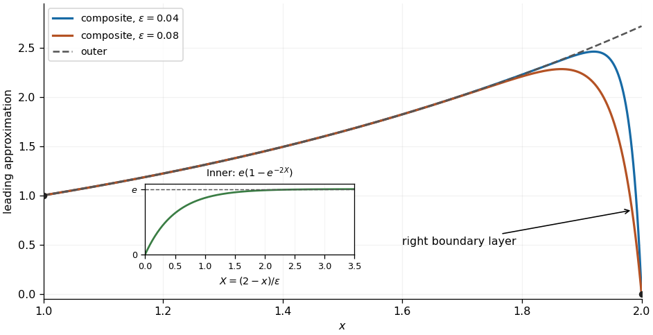
The common value in the overlap region is $e$. The additive composite expansion therefore givesThis leading approximation has $y_{\mathrm{comp},0}(2)=0$ and $y_{\mathrm{comp},0}(1)=1-e^{1-2/ϵ}$; the left endpoint error is exponentially small. It rises from near one following the outer solution $e^{x-1}$, approaches a value close to $e$, then drops rapidly to zero in the right boundary layer. Its first derivative isFor small $ϵ$ the largest value lies slightly inside the interval. For this additive composite expansion, the first derivative vanishes atThis locates the rounded top of the sketch; the rapid final drop has the $O(ϵ)$ scale found above. The additive composite expansion is a leading approximation, so its exponentially small endpoint error does not imply an exponentially small error throughout the interval: neglected algebraic corrections to the outer expansion and inner expansion remain.

The reduced equation and the left boundary condition give the leading outer solutionIntroduce the right inner variable $X=(2-x)/ϵ\ge 0$ and write $Y(X)=y(2-ϵX)$. The chain rule gives $y^{\prime }=-Y_X/ϵ$ and $y^{\prime \prime }=Y_{XX}/{ϵ}^2$. Multiplying the rescaled differential equation by $ϵ$ gives the exact equationAt leading order, $Y_{0,XX}+2Y_{0,X}=0$, with general solution $Y_0=A+B{e}^{-2X}$. The right boundary condition gives $Y_0(0)=0$. The asymptotic matching condition in the overlap region $ϵ\ll 2-x\ll 1$ givesThus $A=e$ and $B=-e$, yielding the leading inner expansionEquivalently, the inner variable $\xi =2(2-x)/ϵ$ gives $Y_0=e(1-e^{-\xi })$. Both normalizations describe the same boundary layer.

Assume $ϵ\downarrow 0$ and fixed $A>0$. Away from the degenerate endpoint $x=0$, the reduced equation is $A{y}_0^{\prime }+y_0=0$. The positive drift makes the rapidly varying homogeneous mode decay as one moves away from the left boundary, so the outer solution is selected by the right boundary condition:It does not satisfy the left value: its limit there is $L=e^{1/A}$.

If the layer width is $\delta$, diffusion is $O(ϵ/{\delta }^2)$, while $Ax{y}^{\prime }$ is $O(A)$ because the drift vanishes linearly. Their dominant balance gives the square-root boundary layer at a vanishing driftWriting $y=Y(\xi )$ gives $Y^{\prime \prime }+\xi Y^{\prime }+[\sqrt{ϵ}/A^{3/2}]\xi Y=0$. The first nonzero inner expansion satisfies $Y_0^{\prime \prime }+\xi Y_0^{\prime }=0$, hence $Y_0^{\prime }=B{e}^{-{\xi }^2/2}$. Imposing $Y_0(0)=1$ and matching $Y_0(\infty )=L$ givesThe overlap region is $\sqrt{ϵ/A}\ll x\ll 1$ for fixed $A$. The additive composite expansioncombines the two leading approximations and satisfies the left value exactly and the right value up to an exponentially small term. Only the first nonzero terms were requested; higher matching terms need not be added.

For fixed $A<0$, the decaying fast mode is at the other endpoint. The outer solution is now fixed by $y(0)=1$, giving $e^{-x/A}$. At $x=1$ the drift does not vanish, so the right layer has width $O(ϵ/|A|)$, with leading transient proportional to $e^{-|A|(1-x)/ϵ}$. In particular its leading inner profile is $e^{-1/A}+(1-e^{-1/A})e^{-\eta }$, where $\eta =|A|(1-x)/ϵ$. The vanishing drift at the left endpoint does not require an order-one mismatch layer for these data.

For $A=0$, the reduced equation is $x{y}_0=0$, which cannot supply the nonzero endpoint values. The equation becomes an Airy ordinary differential equation: $x={ϵ}^{1/3}\xi$ gives $Y^{\prime \prime }+\xi Y=0$. The exact solutions are combinations of $\mathrm{Ai}(-x/{ϵ}^{1/3})$ and $\mathrm{Bi}(-x/{ϵ}^{1/3})$. For $x>0$ they oscillate, with local wavelength of order $\sqrt{ϵ/x}$, rather than forming a decaying exponential layer matched to a smooth nonzero outer profile. The $O({ϵ}^{1/3})$ region resolves the turning endpoint, but oscillations extend throughout the interval. Boundary-value resonances can occur at isolated parameter values. Thus setting $A=0$ is not a continuous substitution into either fixed-sign layer approximation.

The small denominator lies near $x=0$ when $\gamma$ approaches $1$. Its two contributions balance when $\gamma -1=O(\epsilon )$ and $x=O(\epsilon )$. Letwith fixed real $\eta$. Then $1-\gamma +\gamma x=\epsilon (s-\eta )+O({\epsilon }^2)$ and $\log (2-x)=L+O(\epsilon s)$ in the contributing region. The endpoint transition of a regularized interior pole givesIndeed, the leading scaled integral is ${\epsilon }^{-1}{\int }_0^{\infty }[(s-\eta {)}^2+L^2{]}^{-1}ds$. The upper endpoint can be sent to infinity at leading order because the omitted tail contributes only $O(1)$ to the original integral. At $\gamma =1$ the result is $\pi /(2\epsilon \log 2)$: only one half of the narrow peak lies in the domain.

This formula provides the required matching. For $\eta \to -\infty$, $\pi /2+\arctan (\eta /L)\sim -L/\eta$, giving $I\sim 1/(1-\gamma )$. For $\eta \to +\infty$ it tends to $\pi$, giving $I\sim \pi /(\epsilon \log 2)$, the $\gamma \downarrow 1$ limit of the interior-peak approximation. These are overlap regions with $\epsilon \ll |\gamma -1|\ll 1$, not assertions that the fixed-$\eta$ remainder is uniform to arbitrarily large $\eta$.

Write $H(x^{\prime })=h^{\prime }(x^{\prime })$ and $p_x^{\prime }=d{p}^{\prime }/d{x}^{\prime }$ below, so the subscript $x$ in this shorthand denotes differentiation with respect to $x^{\prime }$. The vertical pressure gradient is zero, and integrating $u_{z^{\prime }{z}^{\prime }}^{\prime }=p_x^{\prime }$ twice with the wall boundary conditions gives the local Couette-Poiseuille flowThe first two terms are Couette flow due to the moving plate; the last is plane Poiseuille flow due to the local pressure gradient. Its dimensionless volume flux per unit width isUse the Leibniz integral rule and incompressibility to differentiate this integral:Thus the flux is independent of position, andThe normal velocity can then be recovered from incompressibility:It is zero on the lower wall by construction and zero on the upper wall by the constant-volume flux relation. This supplies the remaining component of the leading velocity field.

The endpoint pressure conditions are matching conditions, not an assertion that the lubrication approximation remains valid at arbitrarily large dimensional $x$. On an outer length scale $R$, a viscous pressure variation is of size $\mu U/R$, whose ratio to the inner scale isEven an outer inertial pressure scale $\rho U^2$ has ratioConsequently the gap pressure is much larger than either outer variation. Matching to fluid with a common ambient pressure at both ends, and taking that value as zero gauge pressure, givesThere is an overlap region $1\ll |x^{\prime }|\ll {\delta }^{-1}$ before the wall slope becomes order one. The infinite endpoints represent matching through that region. An externally imposed pressure difference comparable with $P$ would change these conditions and the resulting volume flux; equal outer pressure is the physical assumption being used here.