where a,b,c are integration constants. Equivalently z−2x and y−z2/4 are constant along each curve: differentiating them with respect to s gives zero. Three constants occur because shifting the origin of the parameter s describes the same geometric curve again; there are two independent curve invariants.
Use t≥0 to label the initial half-line, with (x,y,z)=(t,−t,1) at s=0. In the general characteristic from part (i), this sets a=t, b=−t, c=1. The parametric solution surface is therefore
At s=0 this recovers exactly the given data. Moreover (xs,ys,zs)=(1,1+2s,2)=(1,z,2), so the surface follows the required characteristic vectorfield. The branch defining a classical graph through the data is determined below by restricting to the side of the projection fold containing s=0.
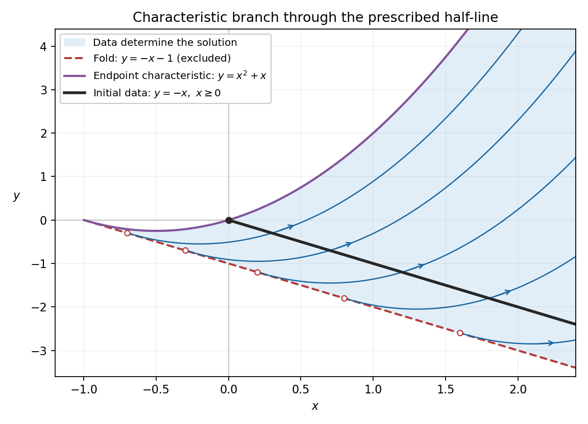
Equality occurs at s=−1, where the point is (t−1,−t). Also dy/dx=ys/xs=1+2s=−1 there, so the tangent line has the same slopeas the line x+y=−1 and passes through a point of that line. Thus every projected characteristic is tangent to that line, with no crossing of it. Because t≥0, the attained tangency points form only the half-line x≥−1, y=−x−1.
It vanishes exactly when s=−1. The image is the tangency half-line from part (iii), x=t−1, y=−t, t≥0. This is a fold caustic: the parameterized surface itself remains regular, but its projection ceases to be locally invertible, so it cannot there be expressed asa differentiable single-valued graph over the plane.
Put W=1+x+y. The identity W=(s+1)2 gives s=−1±W, and hence z=−1±2W. On the initial half-line W=1 and the prescribed value is z=1, which selects the positive sign. The branch containing the data has s>−1, so
On the data y=−x, the value is one. The other algebraic branch gives z=−3 there and does not meet these data. The positive-branch formuladefinesa solution on the larger half-plane W>0, but the part uniquely fixed by the prescribed half-line also requires a nonnegative characteristic footpoint t, as part (vi) explains.
The square root must be positive, and t≥0 requires x+1≥1+x+y>0. Squaring is now legitimate and gives y≤x2+x. Thus the full characteristic-covered set on this branch is
Each point of D has exactly one backward characteristic meeting the interior t>0 of the prescribed data, so the Picard-Lindelöf theorem fixes its value. The upper boundary is the characteristic issuing from the endpoint t=0 and is fixed by the endpoint datum, consistently with the continuous trace from D. The lower boundary is excluded: s=−1 there, the Jacobian determinant vanishes, and the explicit solution derivatives diverge as W↓0.
Points of the half-plane W>0 outside this set have t<0 on the branch through the data. Their characteristic footpoints would lie on the unprescribed continuation of the initial line, so these values are not determined by the given half-line alone. For example, extend the initial value to negative tas 1+εh(t), where h is a smooth function supported on the negative half-line. Such extensions agree with all the prescribed data and, where noncharacteristic, produce different local extensions by the method of characteristics. The displayed formula supplies one possible extension there, but the data do not select it uniquely. This is why retaining the restriction on the initial half-line is essential. Continuing the parameterized surface past s=−1 instead produces the other sheet of the fold; it does not give a differentiable graph continuation through the caustic.