Answer availability checked on 28 October 2026: a bounded search of official Oxford sources found no advertisement of complete or selected-part solutions for this exact paper. The general advertisement of even-year solutions dating back to at least 2016 does not establish coverage of 2012.[ref]
is linearly independent. Its linear spanW is invariant under T: all but the last basis candidate map to the next, and the last maps to Tkv∈W. Induction therefore puts every Tjv in W. Cyclicity gives W=V, so B is a basis and k=n.
For p(t)=tn+an−1tn−1+⋯+a0, the defining relation says p(T)v=0. Since p(T) commutes with T, it also annihilates every Tjv in B, hence p(T)=0. No nonzero polynomial of degree less than n can annihilate v, because that would contradict linear independence of B. Thus mT=p.
Use the inner product convention that the first argument is linear and the second is conjugate-linear. This is the convention corresponding to the conjugated eigenvalue in part (c).
The coefficients are in this order because the inner product is linear in its first argument. For i<k, taking the inner product with qi gives ⟨uk,qi⟩=0. The residual uk cannot be zero: otherwise ek would belong to the linear span of e1,…,ek−1, contradicting the initial basis. Normalization makes ∥qk∥=1, while induction preserves
In an orthonormal basis, every vectorw has the coordinate expansion w=∑i⟨w,ei⟩ei. If ⟨Su,v⟩=⟨u,Rv⟩ for all u,v, apply it to u=ei, v=ej and take complex conjugates:
A Euclidean domain is an integral domainR with a functiond:R∖{0}→N0 such that, for a∈R and nonzero b∈R, there exist q,r∈R with a=qb+r and either r=0 or d(r)<d(b). This is the Euclidean-ring convention used here.
If an idealI is zero, it is generated by zero. Otherwise choose nonzero a∈I with d(a) minimal. For any b∈I, Euclidean division gives b=qa+r, with r∈I. A nonzero remainder would have d(r)<d(a), contradicting the choice. Hence r=0 and b∈aR. The reverse inclusion follows from a∈I, proving
Now suppose a is an irreducible element. Its principal ideal is proper because a is not a unit. If aR⊆J⊆R, write J=bR by the result just proved. Then a=bc for some c∈R. Irreducibility gives either ba unit, so J=R, or ca unit, so bR=aR. There is no intermediate proper ideal, and therefore aR is a maximal ideal.
These two quadratic fields are not isomorphic. In L, the class of Xsquares to −1. But K2 embeds in R by sending its class of X to 2: evaluation at 2 has kernel (X2−2), by irreducibility and polynomialdivision. No real numbersquares to −1, so no element of K2 does. A field isomorphism preserves one, minus one and squaring, so it cannot carry L to K2.
Here the contour and its enclosed region lie in U; the contour can be taken piecewise continuously differentiable. More generally, the same formula needs only holomorphic function on an open neighbourhood of that closed region. The orientation is counterclockwise, so the winding number about an interior point is one.
Write M=∣f(z0)∣. The local maximum property gives a disk around z0 on which ∣f∣≤M, contained in the unit disk. If M=0, then f=0 on that neighbourhood, and the identity theorem makes f zero on the connected unit disk.
Either equality condition says that the holomorphic functionh from part (i) has modulus one at an interior point: at zero in the derivative case, or at the given nonzero point in the other case. Since ∣h∣≤1 everywhere, the maximum modulus principle makes ha constant w with ∣w∣=1. Therefore
The integration circle is counterclockwise. The series converges absolutely at every point of the annulus and uniformly on every compact subannulus. The coefficientintegrals are independent of the choice of ρ by the Cauchy integral theorem applied between two such circles. These statements include R=0 or S=∞ when the indicated annulus has those endpoints.
Equivalently, the Laurent serieshas a finite nonzero principal part, with lowest power exactly (z−z0)−n. Thus (z−z0)nf(z) extends holomorphically with nonzero value at z0; using a smaller positive power would not remove the singularity.
The different Laurent series reflect different annuli separated by the pole at one. Both follow from absolutely convergent geometric series in their stated regions.
If H(0)=0, the function H is not identically zero, since it is nonzero on the punctured disk. The Taylor series and identity theorem give a finite zero order k≥1, so H(z)=zkq(z) with q holomorphic and q(0)=0. Hence
Although the change of variable has an infinite endpoint, the original integrand is continuous on the closed interval, and the transformed integrand decays as u−2, so the limiting substitution is justified.
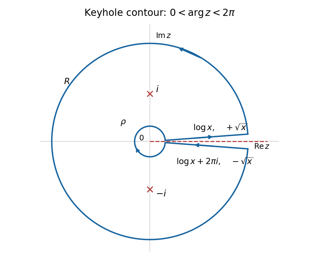
On the upper bank, Logx=logx and x is positive. On the lower bank, the corresponding limits are logx+2πi and −x. Reversing the lower-bank orientation therefore makes the sum of the bank integrals tend to
Both are absolutely convergent: near zero compare with x−1/2(1+∣logx∣), and near infinity with x−5/2(1+logx). On the large circle, ∣z2+1∣≥R2−1, so its contribution is O((logR+1)R−3/2). On the small circle it is O(ρ(1+∣logρ∣)). Both tend to zero.
Both linear modes grow forward in time. Nearby nonconstant orbits move away from the equilibrium, and approach it under reversed time; their local directions come from the two real eigenvectors.
In suitable real coordinates the radius decays like eαt while the angle changes at rate β. The orbit therefore spirals towards the equilibrium, which is asymptotically stable. This is also called a stable focus.
Rotation is accompanied by exponentially increasing radius in suitable real coordinates. Thus nearby nonconstant orbits spiral away, and the equilibrium is unstable. This is also called an unstable focus.
The first component of the vector field vanishes only when y=0 or x=±1. The second vanishes only when y=1 or x+y=3. Intersecting these alternatives gives exactly five equilibria. Their Jacobian matrix is
have one weak sign throughout D, without vanishing identically on any nonempty open subset, then there is no nonconstant periodic orbit contained in D. To see why, a hypothetical simple periodic orbit bounds a region in D. The divergence theorem gives the integral of this expression as the outward flux of B(P,Q) across the orbit. The flux is zero because the vectorfield is tangent to its orbit, whereas the one-signarea integral is nonzero, acontradiction. The usual stricter version assumes a strictly positive or strictly negative expression everywhere.
On the open disk x2+y2<3 this is nonpositive, and is negative wherever x=0. Its zero set inside the disk is a line, so it cannot vanish on any open subset. The Bendixson-Dulac theorem therefore proves
There are no nonconstant periodic orbits contained in x2+y2<3.
For clarity, the quartic terms come from −x4 in the derivative of r2/2, and from applying y∂x−x∂y to the quartic correction. Their sum is −3x4/8−3x2y2/4−3y4/8; all other terms have degree at least six. Therefore V˙<0 in a sufficiently small punctured neighbourhood, proving asymptotic stability by Second Lyapunov theorem. Finally
Indeed, for t<x the kernel is −e2(t−x)sintcosx, since sin(x−t)−sinxcost=−cosxsint; for x<t it is −e2(t−x)sinxcost.
For fixed interior t, the Green's function vanishes at both endpoints, is continuous at x=t, solves the homogeneous equation away from t, and satisfies
It vanishes at zero and at π/2. To check the differential equation directly, set y=e−2xw. Then Ly=e−2x(w′′+w). For w=1−sinx−cosx, one has w′′+w=1, as required.
At x=π, the homogeneous term vanishes for every C; it can no longer be chosen to correct the final boundary value. Since sin(π−t)=sint, that boundary value is zero exactly when
For complex-valued forcing, allow C∈C instead. The freedom is addition of the nonzero homogeneous Dirichlet solution e−2xsinx. At this endpoint separation, the homogeneous boundary problem has a nonzero solution. The resulting Fredholm solvability condition restricts the forcing to the compatible functions described above. In the language of the Fredholm alternative, the condition is orthogonality to the adjoint null solution e2xsinx of D2−4D+5 with zero endpoint values.
A solution surface is locally a differentiable graph z=u(x,y) whose tangent plane contains the vector(P,Q,R) at every point. Its normal is (−ux,−uy,1), so the tangency condition is precisely Pux+Quy=R. Thus every characteristic lying on that graph follows the vectorfield without leaving the graph.
where a,b,c are integration constants. Equivalently z−2x and y−z2/4 are constant along each curve: differentiating them with respect to s gives zero. Three constants occur because shifting the origin of the parameter s describes the same geometric curve again; there are two independent curve invariants.
Use t≥0 to label the initial half-line, with (x,y,z)=(t,−t,1) at s=0. In the general characteristic from part (i), this sets a=t, b=−t, c=1. The parametric solution surface is therefore
At s=0 this recovers exactly the given data. Moreover (xs,ys,zs)=(1,1+2s,2)=(1,z,2), so the surface follows the required characteristic vectorfield. The branch defining a classical graph through the data is determined below by restricting to the side of the projection fold containing s=0.
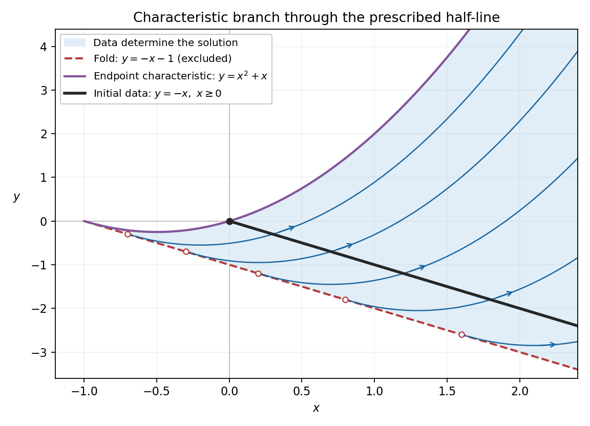
Equality occurs at s=−1, where the point is (t−1,−t). Also dy/dx=ys/xs=1+2s=−1 there, so the tangent line has the same slopeas the line x+y=−1 and passes through a point of that line. Thus every projected characteristic is tangent to that line, with no crossing of it. Because t≥0, the attained tangency points form only the half-line x≥−1, y=−x−1.
It vanishes exactly when s=−1. The image is the tangency half-line from part (iii), x=t−1, y=−t, t≥0. This is a fold caustic: the parameterized surface itself remains regular, but its projection ceases to be locally invertible, so it cannot there be expressed asa differentiable single-valued graph over the plane.
Put W=1+x+y. The identity W=(s+1)2 gives s=−1±W, and hence z=−1±2W. On the initial half-line W=1 and the prescribed value is z=1, which selects the positive sign. The branch containing the data has s>−1, so
On the data y=−x, the value is one. The other algebraic branch gives z=−3 there and does not meet these data. The positive-branch formuladefinesa solution on the larger half-plane W>0, but the part uniquely fixed by the prescribed half-line also requires a nonnegative characteristic footpoint t, as part (vi) explains.
The square root must be positive, and t≥0 requires x+1≥1+x+y>0. Squaring is now legitimate and gives y≤x2+x. Thus the full characteristic-covered set on this branch is
Each point of D has exactly one backward characteristic meeting the interior t>0 of the prescribed data, so the Picard-Lindelöf theorem fixes its value. The upper boundary is the characteristic issuing from the endpoint t=0 and is fixed by the endpoint datum, consistently with the continuous trace from D. The lower boundary is excluded: s=−1 there, the Jacobian determinant vanishes, and the explicit solution derivatives diverge as W↓0.
Points of the half-plane W>0 outside this set have t<0 on the branch through the data. Their characteristic footpoints would lie on the unprescribed continuation of the initial line, so these values are not determined by the given half-line alone. For example, extend the initial value to negative tas 1+εh(t), where h is a smooth function supported on the negative half-line. Such extensions agree with all the prescribed data and, where noncharacteristic, produce different local extensions by the method of characteristics. The displayed formula supplies one possible extension there, but the data do not select it uniquely. This is why retaining the restriction on the initial half-line is essential. Continuing the parameterized surface past s=−1 instead produces the other sheet of the fold; it does not give a differentiable graph continuation through the caustic.