Original solutions to all three questions of the Approximation of Functions paper sat on 16 June 2011. Source: released Mathematics papers,
Part C 2007 11.pdf. Question 3 includes a counterexample to the unqualified printed endpoint exchange rule and the corrected rule. Statements are not reproduced.The Lagrange interpolation polynomial isThe interpolation nodes are distinct, so these weights are well defined. Applying the same Lagrange interpolation to the constant polynomial one gives . Dividing this identity and the formula for by gives the barycentric interpolation formulaThis displayed quotient is used away from the interpolation nodes; at its removable singularity is evaluated by setting . Multiplying every weight by the same nonzero constant leaves the quotient unchanged.
Chebyshev points are generally more reliable at high degree. The Chebyshev-Lobatto nodes, or the affine images of the roots of a Chebyshev polynomial, cluster near the interval endpoints and control the amplification measured by the Lebesgue constant of interpolation. Equally spaced interpolation nodes can produce large endpoint oscillations and the Runge phenomenon. This is a comparison of numerical robustness and general approximation behaviour, not a claim that one set minimizes the error for every individual function.
Assume . The functional is the third forward difference: each forward difference lowers the polynomial degree by one, so it annihilates every polynomial of degree at most two. Directly, , , and .
The Peano kernel theorem now gives , where the Peano kernel of the third forward difference isHere is the positive-part truncated power function. The normalized quadratic cardinal B-spline isIts three polynomial pieces agree with the displayed kernel after rescaling, giving . Its knots are in the physical variable, and is positive throughout .
The kernel mass can be evaluated without integrating each piece: apply its representation to , whose third derivative is one. This gives . The weighted mean value theorem for integrals with a nonnegative weight therefore yieldsContinuity of and strict positivity of the weight in the interior place an attained weighted-average value in that open interval, including the constant-derivative case.
Take , as intended by the stated normalization. The Chebyshev polynomial recurrence , with and , shows by mathematical induction that has polynomial degree and leading coefficient . Consequently is a monic polynomial. At the ordered Chebyshev extreme points ,and .
Suppose a monic polynomial of the same polynomial degree had . The difference has degree at most because its leading coefficients cancel. Its signs at the ordered extreme points strictly alternate. The intermediate value theorem supplies a distinct root of a polynomial between each consecutive pair, giving at least roots. This contradicts its degree bound. Hence the monic Chebyshev extremal polynomial satisfiesAt the printed formula instead gives , which is not monic; the degree-zero minimizer is the constant one. This endpoint case requires the separate normalization .
Put in the weighted inner product. Since ,The last equality follows by the product-to-sum trigonometric identity and integration. Thus these are nonzero mutually orthogonal polynomials. The first are linearly independent, and the vector space has dimension ; therefore .
For any , the function of the real parameter has a minimum at . Its derivative there vanishes, proving . This is precisely the defining orthogonality of an orthogonal projection, or a least-squares polynomial in an orthogonal-polynomial basis. Conversely, this condition and the Pythagorean theorem for inner product spaces give , proving the minimum and its uniqueness.
Expand in the basis already established and take the inner product with . Orthogonality leaves , soIn particular and for . These are the corresponding Chebyshev series coefficients with the constant coefficient convention used in this question.
The equioscillation theorem says that is the unique best uniform approximation to a real continuous function on exactly when its error attains alternating values at ordered distinct points. If , the error vanishes everywhere and the conclusion is immediate.
For the exponential function, write the candidate line as . Its error is strictly convex. Equal endpoint errors require , and the interior minimum is at , because . Equating the endpoint error to the negative interior error givesIndeed and ; convexity puts every other error value between these extremes. The equioscillation theorem proves optimality.
For the reference-point assertions, put . The alternating-reference error bound gives . In fact this inequality is strict here. To see the equality obstruction explicitly, let be optimal, , andSince has polynomial degree at most , its order- divided difference vanishes: . If , change the overall sign to take . The error bound for implies . The signs of the weights are , so every term in this sum has the same weak sign. Every term must vanish; then has distinct zeros, forcing . This contradicts . If , and the same zero-count argument again forces , also a contradiction. ThusAt every old reference point the absolute error is only , so a maximizer cannot be one of those points. The printed same-sign choice of additionally presumes ; when , none of the reference errors has the nonzero sign of the maximal error.
The printed replacement rule needs an endpoint qualification. For an interior and nonzero , replacing the adjacent endpoint of its containing reference interval with the same error sign preserves spatial order and alternating signs. The single-point exchange in polynomial minimax approximation then gives the requested strict increase. On an irregular grid, the globally nearest same-sign reference point need not be that adjacent endpoint, so adjacency must be specified. More generally, for any correctly ordered replacement set on which the old error alternates in sign, let . The vanished divided difference of and the new alternation equations showThis is a strict weighted average because all the weights are positive in absolute value and .
For an exterior whose error sign is opposite that at the nearest endpoint, merely replacing the nearest same-sign point, as printed, need not preserve alternation. A concrete counterexample uses , , , and reference pointsLet be the piecewise linear function through . Then at , and : the upper bound is achieved by the trial constant , while equality at the lower bound is excluded by the preceding zero-count argument. The printed rule selects and hence . Neverthelesssatisfy every printed new alternation equation, with . Direct substitution at the four points checks this failure; reordering those points would destroy their assigned alternating signs.
The corrected exterior rule inserts as the new extreme reference point and drops the farthest endpoint when its sign is opposite the nearest endpoint. If its sign agrees with the nearest endpoint, replace that endpoint. Interior exchanges replace the adjacent reference point with the same sign. These rules preserve an ordered alternating set, so the strict-increase formula applies in every case.
The resulting Remez algorithm solves the linear alternation equations for the polynomial coefficients and reference height, locates a global maximum of the error, and performs a valid exchange unless . The interval is an explicit optimality certificate; a small gap gives a stopping test. Strict increase of bounded reference heights alone does not prove convergence, so that stronger conclusion needs the additional analysis of the chosen exchange algorithm.
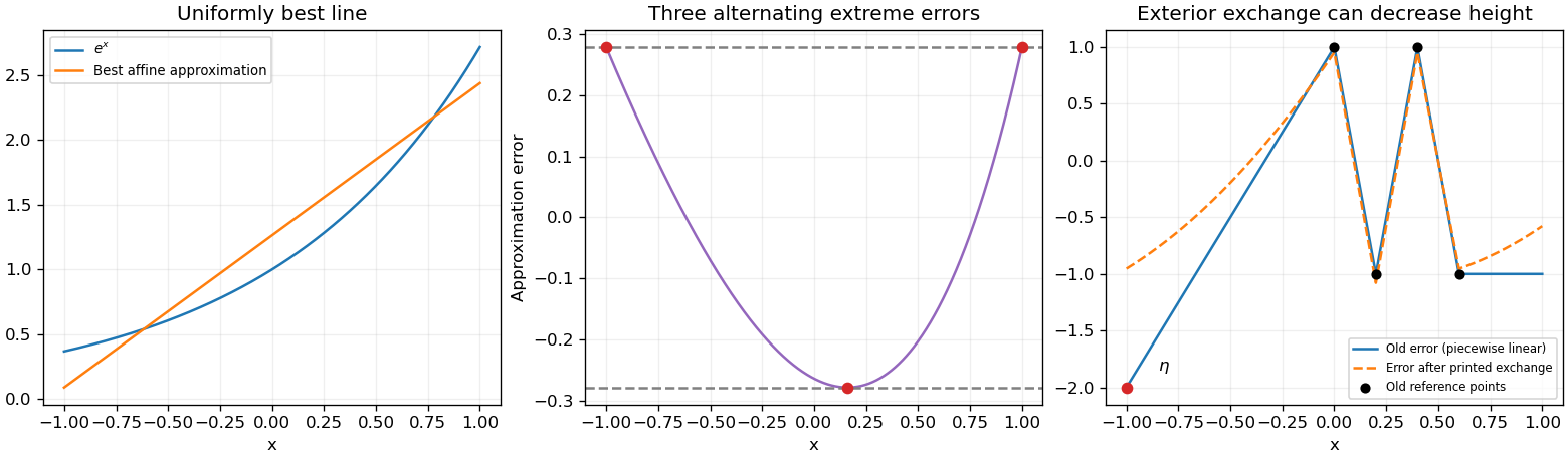
Minimax linear approximation to the exponential and a counterexample to the unqualified exterior exchange rule
. Details. 
Articles by others on the same topic
There are currently no matching articles.