Past exam of the differential equations 1 course of the University of Oxford / 2017 / 2

The contraction mapping theorem states that a contraction mapping $T:S\to S$ on a nonempty complete metric space has a unique fixed point. Explicitly, if $d(Tu,Tv)\le qd(u,v)$ for all $u,v\in S$ and one fixed $0\le q<1$, then the iterates $u_{n+1}=T{u}_n$ converge to that fixed point from every $u_0\in S$. Both self-mapping and completeness are needed; the set need not be a vector space.

For $0<\eta \le h$, work on the closed subsetIt is a nonempty complete metric space because it is closed in the Banach space of continuous functions with the supremum norm. Define the Picard iteration operatorChoose $\eta$ so that $M\eta \le k$ and $L\eta <1$, omitting a bound whose constant is zero. Such a positive $\eta$ exists. The first inequality makes $T$ a self-map, since $|(Ty)(x)-b|\le M|x-a|\le k$. The Lipschitz condition givesso the contraction mapping theorem yields a unique fixed point. The fundamental theorem of calculus makes it a differentiable solution of $y^{\prime }=f(x,y)$ with $y(a)=b$; conversely every solution staying in the rectangle satisfies the integral equation and is a fixed point. This is the local Picard-Lindelöf theorem construction. The interval-restricted space $C_{\eta }$ avoids treating functions defined on a shorter interval as elements of $C_h$.

Under $Mh\le k$, the same Picard iteration operator maps all of $C_h$ into itself. It need not be a contraction mapping in one step, since $Lh$ can exceed one. Instead repeated integration gives the factorial estimate for Picard iterationproved inductively by integrating the preceding bound between $a$ and $x$. ThusFor some $n$ the coefficient is less than one, so $T^n$ is a contraction. Its unique fixed point $y_{\ast }$ is also fixed by $T$: $T^n(T{y}_{\ast })=T(T^n{y}_{\ast })=T{y}_{\ast }$ and uniqueness forces $T{y}_{\ast }=y_{\ast }$. Conversely any fixed point of $T$ is one of $T^n$. This iterated contraction argument gives a unique solution on the full interval $[a-h,a+h]$, without the unjustified extra assumption $Lh<1$.

The uniqueness statement is for solutions in the specified rectangle, where $f$ is given and controlled. The bound $Mh\le k$ keeps the constructed solution inside that rectangle throughout the interval.

Where $y\ne -1$, $y^{\prime }=-\sqrt{|1+y|}<0$. By the mean value theorem, the solution is strictly decreasing on every interval where it avoids $-1$. At $y=-1$, the derivative is zero, so a constant segment there is possible. Thus all solutions are nonincreasing, while strict decrease need not persist through an interval spent at that equilibrium.

For example, choose $h=1/4$ and $k=1/2$ around $(a,b)=(0,0)$. On the rectangle, $1+y\ge 1/2$, so $f=-\sqrt{1+y}$ is continuous, $|f|\le \sqrt{3/2}$ and $|\partial f/\partial y|\le 1/\sqrt{2}$. The mean value theorem therefore supplies a Lipschitz constant $L=1/\sqrt{2}$. These choices even satisfy $Mh<k$ and $Lh<1$.

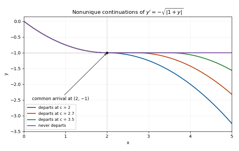
While $y>-1$, separation of variables gives $2\sqrt{1+y}=2-x$. Therefore the uniquely determined branch up to its first arrival at $-1$ isIt reaches $y=-1$ at $x=2$, with derivative zero. The restriction $x\le 2$ is essential: extending the same quadratic beyond two would make its derivative positive and violate the original differential equation. Beyond that time the waiting-time continuation at a non-Lipschitz equilibrium is nonunique.

Two solutions for $x\ge 2$ areFor the second, $y_2^{\prime }=-(x-2)/2=-\sqrt{|1+y_2|}$ because $x\ge 2$; both have value $-1$ and derivative zero at two. They are distinct for every $x>2$. Local Lipschitz continuity fails at the equilibrium, so the existence of these two continuations is compatible with the Picard-Lindelöf theorem.

For each departure time $c\in [2,h]$, defineEach branch satisfies the ordinary differential equation, and both joins have matching value $-1$ and matching derivative zero. Thus $y_c$ is continuously differentiable and satisfies the same initial value problem. If $2\le c_1<c_2\le h$, the solutions differ on $(c_1,c_2)$, proving infinitely many solutions on every $[0,h]$ with $h>2$.

The uniqueness hypotheses fail when the solution reaches $-1$. IndeedNo finite Lipschitz constant works on a rectangle containing that level in its interior. The local theorem still controls the earlier branch near zero; it cannot be extended through a point where its hypotheses fail. These are waiting-time continuations at a non-Lipschitz equilibrium.