Past exam of the differential equations 1 course of the University of Oxford / 2017 (A15294W1, A1)

Source paper: released examination archive, member 2016/T/a15294w1.pdf. The printed cover dates the examination to 16 June 2017. All three questions and all eighteen terminal subparts, including the two displayed cases in part 3(d), are answered below.

The autonomous planar system has two real state variables, so its phase space is a subset of ${\mathbb{R}}^2$. It is autonomous because its vector field $(X(x,y),Y(x,y))$ has no explicit time dependence. The nullclines are $X(x,y)=0$ and $Y(x,y)=0$, on which the respective coordinate's instantaneous rate of change vanishes. A critical point of a dynamical system is an intersection where $X=Y=0$; the constant trajectory at that point is an equilibrium of an autonomous differential equation. A nullcline alone need not consist of equilibria.

Assume $X,Y$ are continuously differentiable near the equilibrium. Put $\xi =x-a$, $\eta =y-b$ and expand the vector field:This Jacobian matrix defines the linearized system. For distinct real eigenvalues, two negative values give a stable node, two positive values an unstable node, and opposite signs a saddle point of a dynamical system. A complex-conjugate pair with negative real part gives a stable focus, and one with positive real part an unstable focus. Thus a hyperbolic saddle has two real eigenvalues of opposite signs, equivalently $\det M<0$.

The linearization stability theorem transfers these stability conclusions to the nonlinear system when no eigenvalue has zero real part. Distinctness alone is insufficient: a zero eigenvalue or a purely imaginary conjugate pair leaves a nonhyperbolic equilibrium, for which the nonlinear terms must be examined. In the purely imaginary case the linearized trajectories form a centre, but that does not establish a nonlinear centre.

One useful form of the Bendixson-Dulac theorem is this: let $D\subseteq {\mathbb{R}}^2$ be open and simply connected, and let $X,Y,\psi$ be continuously differentiable on $D$. Ifhas one strict sign throughout $D$, then there is no nonconstant periodic orbit lying entirely in $D$. More generally the divergence may have a weak sign provided it is not identically zero on any nonempty open subset. The multiplier $\psi$ is a Dulac function. Green's theorem proves the criterion: the vector field is tangent to a hypothetical closed orbit, so its scaled flux across that boundary is zero, whereas the signed area integral of its divergence would be nonzero.

Intersect the nullclines $y=x(2-x)$ and $y=kx$. Their intersection equation is $x(2-k-x)=0$, giving the origin and $(2-k,k(2-k))$. The Jacobian matrix isAt the origin, $\mathrm{tr}M=3$, $\det M=2-k$ andFor $k>2$, only the origin is in the nonnegative quadrant, and it is a saddle because its determinant is negative. For $0<k<2$, the origin is an unstable node, with two distinct positive eigenvalues, and there is a second equilibrium in the open quadrant. At that second equilibrium, $\det M=k-2<0$, so it is a saddle. These signs give hyperbolic equilibria, so the nonlinear classifications follow from the linearization stability theorem. The boundary value $k=2$ is excluded from the two stated cases.

Draw the downward-opening nullcline $y=x(2-x)$, meeting the axes at $x=0,2$, and the line $y=kx$. Their positive intersection is $P=(2-k,k(2-k))$. Use the sign rulesAbove both curves the arrows point northwest; below both they point southeast. For $0<x<2-k$, the parabola lies above the line, so arrows between them point northeast. For $2-k<x<2$, their order reverses, so arrows between them point southwest. For $x>2$, $\dot{x}<0$ throughout the nonnegative quadrant, with the vertical direction still determined by the line. Mark the origin as an unstable node and $P$ as a saddle, and trace sample trajectories consistent with those directions.

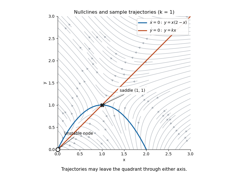
The quadrant is not positively invariant: on $x=0,y>0$, $\dot{x}=-y<0$; on $y=0,x>0$, $\dot{y}=-kx<0$. Trajectories reaching either axis there leave the plotted region. The phase portrait describes the portions inside the quadrant, not a claim that all forward trajectories remain inside it.

Let $k>2$ and choose the positive Dulac functionMore generally, for $\psi =e^{a(x+y)}$, direct differentiation givesTaking $a=-2/(k-2)$ cancels the linear term and makes the quadratic term nonnegative:The open positive quadrant is simply connected, so the Bendixson-Dulac theorem excludes every nonconstant periodic orbit entirely inside it. Such an orbit cannot touch $x=0,y>0$ while staying in the closed quadrant, since its differentiable coordinate $x$ would have a local minimum there but $\dot{x}=-y\ne 0$. The same argument applies on $y=0,x>0$. It cannot pass through the origin either, by local uniqueness of this smooth autonomous system. Therefore there is no nonconstant closed trajectory in the entire nonnegative quadrant. The calculation illustrates an exponential Dulac multiplier for a quadratic planar system.

The contraction mapping theorem states that a contraction mapping $T:S\to S$ on a nonempty complete metric space has a unique fixed point. Explicitly, if $d(Tu,Tv)\le qd(u,v)$ for all $u,v\in S$ and one fixed $0\le q<1$, then the iterates $u_{n+1}=T{u}_n$ converge to that fixed point from every $u_0\in S$. Both self-mapping and completeness are needed; the set need not be a vector space.

For $0<\eta \le h$, work on the closed subsetIt is a nonempty complete metric space because it is closed in the Banach space of continuous functions with the supremum norm. Define the Picard iteration operatorChoose $\eta$ so that $M\eta \le k$ and $L\eta <1$, omitting a bound whose constant is zero. Such a positive $\eta$ exists. The first inequality makes $T$ a self-map, since $|(Ty)(x)-b|\le M|x-a|\le k$. The Lipschitz condition givesso the contraction mapping theorem yields a unique fixed point. The fundamental theorem of calculus makes it a differentiable solution of $y^{\prime }=f(x,y)$ with $y(a)=b$; conversely every solution staying in the rectangle satisfies the integral equation and is a fixed point. This is the local Picard-Lindelöf theorem construction. The interval-restricted space $C_{\eta }$ avoids treating functions defined on a shorter interval as elements of $C_h$.

Under $Mh\le k$, the same Picard iteration operator maps all of $C_h$ into itself. It need not be a contraction mapping in one step, since $Lh$ can exceed one. Instead repeated integration gives the factorial estimate for Picard iterationproved inductively by integrating the preceding bound between $a$ and $x$. ThusFor some $n$ the coefficient is less than one, so $T^n$ is a contraction. Its unique fixed point $y_{\ast }$ is also fixed by $T$: $T^n(T{y}_{\ast })=T(T^n{y}_{\ast })=T{y}_{\ast }$ and uniqueness forces $T{y}_{\ast }=y_{\ast }$. Conversely any fixed point of $T$ is one of $T^n$. This iterated contraction argument gives a unique solution on the full interval $[a-h,a+h]$, without the unjustified extra assumption $Lh<1$.

The uniqueness statement is for solutions in the specified rectangle, where $f$ is given and controlled. The bound $Mh\le k$ keeps the constructed solution inside that rectangle throughout the interval.

Where $y\ne -1$, $y^{\prime }=-\sqrt{|1+y|}<0$. By the mean value theorem, the solution is strictly decreasing on every interval where it avoids $-1$. At $y=-1$, the derivative is zero, so a constant segment there is possible. Thus all solutions are nonincreasing, while strict decrease need not persist through an interval spent at that equilibrium.

For example, choose $h=1/4$ and $k=1/2$ around $(a,b)=(0,0)$. On the rectangle, $1+y\ge 1/2$, so $f=-\sqrt{1+y}$ is continuous, $|f|\le \sqrt{3/2}$ and $|\partial f/\partial y|\le 1/\sqrt{2}$. The mean value theorem therefore supplies a Lipschitz constant $L=1/\sqrt{2}$. These choices even satisfy $Mh<k$ and $Lh<1$.

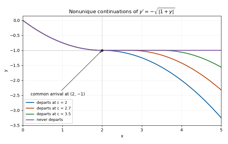
While $y>-1$, separation of variables gives $2\sqrt{1+y}=2-x$. Therefore the uniquely determined branch up to its first arrival at $-1$ isIt reaches $y=-1$ at $x=2$, with derivative zero. The restriction $x\le 2$ is essential: extending the same quadratic beyond two would make its derivative positive and violate the original differential equation. Beyond that time the waiting-time continuation at a non-Lipschitz equilibrium is nonunique.

Two solutions for $x\ge 2$ areFor the second, $y_2^{\prime }=-(x-2)/2=-\sqrt{|1+y_2|}$ because $x\ge 2$; both have value $-1$ and derivative zero at two. They are distinct for every $x>2$. Local Lipschitz continuity fails at the equilibrium, so the existence of these two continuations is compatible with the Picard-Lindelöf theorem.

For each departure time $c\in [2,h]$, defineEach branch satisfies the ordinary differential equation, and both joins have matching value $-1$ and matching derivative zero. Thus $y_c$ is continuously differentiable and satisfies the same initial value problem. If $2\le c_1<c_2\le h$, the solutions differ on $(c_1,c_2)$, proving infinitely many solutions on every $[0,h]$ with $h>2$.

The uniqueness hypotheses fail when the solution reaches $-1$. IndeedNo finite Lipschitz constant works on a rectangle containing that level in its interior. The local theorem still controls the earlier branch near zero; it cannot be extended through a point where its hypotheses fail. These are waiting-time continuations at a non-Lipschitz equilibrium.

The principal coefficients are $A=-xy$, $B=0$, $C=1$, in the convention $A{u}_{xx}+2B{u}_{xy}+C{u}_{yy}$. Their discriminant is $B^2-AC=xy$. Thus it is a hyperbolic partial differential equation where $xy>0$ and an elliptic partial differential equation where $xy<0$. Its principal part has parabolic type where $xy=0$; however the full equation contains $u_y/y$ and is undefined on $y=0$. On its actual domain $y\ne 0$, the parabolic locus is $x=0$.

The characteristic equation of a partial differential equation isIn a hyperbolic region this gives two distinct real characteristic directions. The singular lower-order coefficient should not be mistaken for an ordinary parabolic point of the full equation on $y=0$.

In $x,y>0$, the characteristic equation of a partial differential equation gives $dx/\sqrt{x}=\pm \sqrt{y}dy$. Integration yields the characteristic coordinatesTheir Jacobian determinant is $-\sqrt{y}/(2\sqrt{x})\ne 0$, so they are valid independent coordinates. To see cancellation of the lower-order terms explicitly, first put $r=\sqrt{x}$, $s=y^{3/2}/3$ and $u(x,y)=U(r,s)$. The chain rule givesSubstitution cancels the first-derivative terms, leaving $U_{ss}-U_{rr}=0$. With $\xi =r+s$, $\eta =r-s$ and $U=V(\xi ,\eta )$, the characteristic normal form is $V_{\xi \eta }=0$. Integrating once in each variable giveswhere $g,h$ are arbitrary twice continuously differentiable functions on the relevant coordinate intervals. This is a curvilinear reduction to the one-dimensional wave equation.

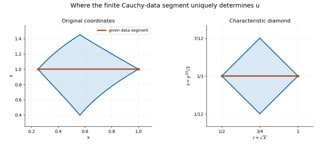
On $y=1$, the transformed variables satisfy $s=1/3$ and $1/2\le r\le 1$. Differentiating the displacement data tangentially and using $u_y=1$ givesHence $g^{\prime }=2$ on $[5/6,4/3]$, $h^{\prime }=0$ on $[1/6,2/3]$, and the additive constants have sum $-2/3$. The uniquely determined solution is thereforeIt is fixed by the data exactly where both needed characteristic arguments belong to their known intervals:Equivalently, in the $(r,s)$ plane this is the diamond $|r-3/4|+|s-1/3|\le 1/4$. In the original coordinates it is bounded by four curved characteristic curves. It lies wholly in $x,y>0$. The displayed formula supplies one smooth extension beyond the diamond too, but the specified finite data segment does not determine that extension: one may change $g$ or $h$ outside its known argument interval. This is the characteristic-coordinate domain of dependence.

The initial curve $y^3=9x$ is $\eta =0$, with $\xi =2\sqrt{x}\in [1,2]$, so it is characteristic. The displacement data force $g(\xi )+h(0)=\xi$ and therefore $g^{\prime }=1$ on that interval. Along the curve,The derivative data in case (i) are compatible precisely when $h^{\prime }(0)=-1$. They place no restriction on the rest of $h$. For example, for every real constant $C$,solves the equation and has both prescribed data on the curve. Choosing $C=0$ and $C=1$ exhibits more than one solution directly. The initial curve follows one characteristic family, so its data do not determine the other wave family. This is the compatible case of compatibility of Cauchy data on a characteristic curve.

As in case (i), the initial curve is characteristic and its displacement data force $g^{\prime }=1$. The new derivative data would therefore requireThe right-hand side varies along the initial segment. A single number $h^{\prime }(0)$ cannot satisfy those conditions, so no classical solution exists.

Characteristic Cauchy data impose a compatibility condition on transverse derivatives without determining the missing independent wave family. Compatible data can leave nonuniqueness, as in case (i); incompatible data have no solution, as here. The distinction follows from compatibility of Cauchy data on a characteristic curve, rather than a noncharacteristic existence-and-uniqueness theorem.