Use dimensionless variables , , , , withSubstitution gives the requested system, with dots now meaning differentiation with respect to , andIn particular the same scale for makes the first two coefficients of the cubic equal in magnitude.
Its derivative is . For its two simple zeros areThe cubic increases below , decreases between the two fold points of a critical manifold, and increases above . It has a local maximum at and a local minimum at .
After a rapidly decaying transient response, when its relaxation is faster than the other variables. The reduced autonomous system isFor , the fast dynamics at fixed attracts to the branches where and repels from the middle branch. On the low branch , increases slowly. At its fold point of a critical manifold , the attracting low branch disappears and jumps upward, with nearly constant , to the high branch. On that branch , decreases slowly. At it jumps back to the low branch. These slow arcs and fast jumps form the singular relaxation cycle. For small positive , and parameters bounded away from the fold point of a critical manifold-endpoint cases, the nearby attracting periodic motion has the same pattern. The equilibrium is on the repelling branch: its Jacobian matrix has determinant and trace .
The limiting landing values are after the upward jump and after the downward jump, obtained from the third root of . Thus the two vertical segments in the phase plane plot really connect roots of the same fast equation.
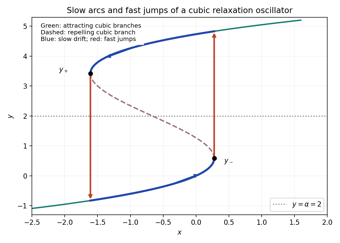
Cubic folds and the singular relaxation cycle: slow drift on attracting branches and fast jumps at nearly fixed x
. Details. 
If , is strictly positive everywhere, so the cubic is monotone and has no fold points of a critical manifold. The reduced equilibrium is asymptotically stable. In factThe only invariant trajectory in the zero-derivative set is the equilibrium, so bounded reduced solutions converge to it; relaxation oscillations disappear.
The stronger condition matters during a fast jump: then varies on the time scale, not on the slow unit scale. Only if adjusts faster still may one keep through that jump. Merely imposing would not justify this reduction on all pieces of the cycle. This is a three-time-scale cubic relaxation oscillator.
For zero damping the conserved mechanical energy isFor , the potential grows to infinity in both directions, so every nonstationary finite-energy trajectory is trapped between two turning points and is periodic; the zero-energy solution is stationary. The case is the harmonic oscillator. The negative- comparison extends the parameter range initially stated in the source.
For , the origin lies in a local potential well, with barriers at of height . A trajectory launched from the origin oscillates precisely when its initial energy is below that barrier:At equality the trajectory approaches a barrier equilibrium asymptotically, rather than being periodic; for example the positive branch is . Above the barrier the trajectory escapes the well. The source's inequality without the absolute value tacitly takes ; for signed initial velocity the energy criterion requires .
Next set and assume . The energy satisfies . This bounds the complete trajectory. The zero-dissipation set is the union of and , and its only invariant trajectory is the origin: a nonzero point on either axis immediately leaves it under the differential equation. The LaSalle invariance principle therefore gives . If as well, damping is absent and that conclusion fails for nonzero ; the positive order-one damping assumption is essential.
For the weakly nonlinear periodic motion, write , set , , and expand . The first correction obeysResonant forcing at the fundamental frequency would generate secular terms. Eliminating both coefficients yieldsConsequently the maximum displacement is for fixed positive . A possible third-harmonic correction is , up to homogeneous amplitude and phase choices. The leading amplitude also balances averaged damping: its slow evolution is , whose nonzero fixed point is attracting. The case is a degenerate zero-amplitude limit, rather than a nonzero limit cycle.
For the singular-endpoint equation, take , , . The indicial equation is . The constant branch violates the zero endpoint value unless its coefficient vanishes; the nontrivial admissible branch therefore has . More precisely, an eigenfunction has and near zero.
Integrate the self-adjoint equation after multiplying by , initially on with :At zero the boundary expression is , the first integrand is , and the second is . Both integrals converge and the boundary term vanishes. Division by the positive weighted norm gives .
The change of coordinate , gives exactlyThus and . To prove a minimum over trial functions, rather than just identify the least eigenvalue, transform the quotient itself:The Dirichlet Poincaré inequality gives the last step, with equality precisely for a nonzero multiple of . The trial class is the nonzero finite-energy class with zero Sobolev traces; endpoint values alone without an integrability requirement do not define a finite quotient. This is the Power-coordinate reduction of a singular Sturm-Liouville quotient.
With diffusion absent, the characteristic equations for a first-order quasilinear equation are , . A characteristic curve labelled by its starting point isThis determines a smooth single-valued solution while is one-to-one. Its derivative isAll characteristic curves move right because . Because , increasing portions of the initial profile have slower characteristic curves ahead than behind, so they steepen. The first positive gradient catastrophe occurs atThis is a minimum when attained. The numerator at such a point is positive and the denominator decreases to zero from above, so .
Resolve the thin transition with and . The leading balance is , where . Integrating once and matching to the state behind givesMatching the state ahead requires and gives the Rankine-Hugoniot speedThe strictly concave graph of has zeros at the two states and lies above its chord, hence is strictly positive between them. Since , through the layer. A heteroclinic profile increasing with can therefore connect the rear state at to the front state at only when . The concavity also gives : characteristic curves enter the viscous shock from both sides. Reversing the states would demand a decreasing profile, contradicting the sign of .
Articles by others on the same topic
There are currently no matching articles.