Past exam of the mathematical physiology course of the University of Oxford / 2011 / 1

In the Hodgkin-Huxley model, $V$ is the membrane potential, the voltage inside the axon relative to outside. The space clamp assumption makes it spatially uniform. The gating variables lie between zero and one: $m$ describes sodium activation, $h$ describes availability against sodium inactivation, and $n$ describes potassium activation. Thus large $h$ means channels remain available, not that inactivation is strong.

The left side $C_m\dot{V}$ is capacitive electric current per unit membrane area. The imposed $I$ is inward-positive applied electric current. The other terms are outward-positive ionic electric currents: sodium with electrical conductance $g_{Na}{m}^{3}h$, potassium with conductance $g_K{n}^4$, and a passive leak with conductance $g_L$. Each current is its conductance times the difference between $V$ and the corresponding reversal potential $V_{Na}$, $V_K$ or $V_L$. The coefficients $g_{Na},g_K$ are maximal conductances; the gate factors represent independent permissive gates in an ion channel.

For each gate, $k_{\infty }(V)$ is the equilibrium opening/availability fraction at fixed voltage and ${\tau }_k(V)>0$ its exponential relaxation time. The equation follows from two-state ion-channel gating: if $\dot{k}={\alpha }_k(V)(1-k)-{\beta }_k(V)k$, thenVoltage feedback couples these otherwise elementary gating equations to the membrane potential and produces action potentials.

Write $M(v)=m^3(v)$. In the physically relevant strip $-v_K<v<1$, $0<n<H$, the zero-current nullcline satisfiesThe left side increases strictly from zero to infinity, so there is exactly one nullcline height $n=N(v)$ for each interior voltage. If $M$ is positive at the endpoints, its curve joins $(-v_K,H)$ to $(1,0)$; when low-voltage activation is idealized as exactly zero, the limiting left branch can lie on $v=-v_K$.

The signs of the derivatives explain its folds:At low voltage, potassium's approximately linear contribution dominates and $g_v>0$. During rapid sodium activation the last negative term can dominate, giving $g_v<0$. Once activation saturates, $M^{\prime }$ becomes small and $g_v>0$ again. This folded conductance-model nullcline has the familiar shape: the curve has descending outer branches and an ascending middle branch in the $(v,n)$ plane. Equivalently, an intermediate fixed $n$ can give three zeros of $g$ as voltage rises, with positive, negative and positive $g_v$ at those crossings.

The rapid-activation description permits this folded shape; exact fold positions depend on $M,{\gamma }_K,H,v_K$. The figure supplies an explicit admissible sigmoid example. Its right panel shows $g=0$ as well as the recovery nullcline and an oscillating trajectory.

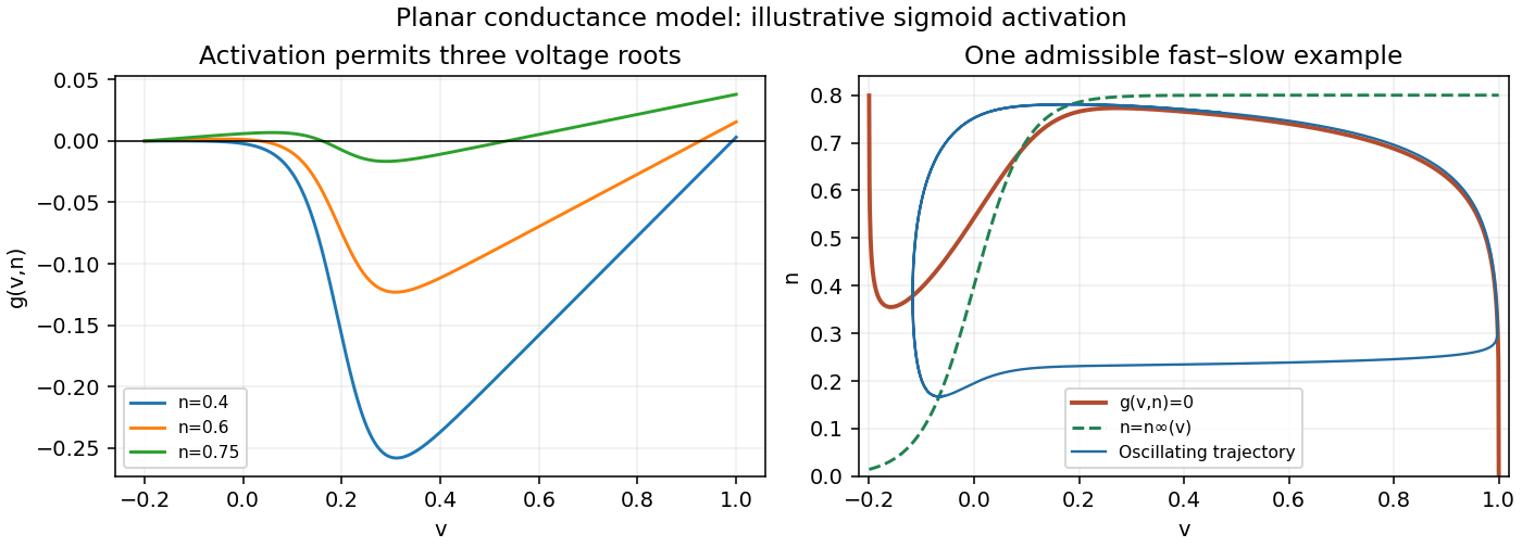
The voltage nullcline is $g(v,n)=I^{\ast }$ and the recovery nullcline is $n=n_{\infty }(v)$. In the relevant region $g_n>0$, so below the voltage curve $\dot{v}>0$ and above it $\dot{v}<0$. Below the recovery curve $\dot{n}>0$, while above it $\dot{n}<0$.

For small $ϵ$, the outer voltage branches with $g_v>0$ attract fast voltage motion; the middle branch with $g_v<0$ repels it. Arrange the intersections so the equilibrium is on that middle branch, with recovery increasing along the high-voltage attracting branch and decreasing along the low-voltage attracting branch. The trajectory then drifts towards a fold, jumps rapidly to the other attracting branch at nearly constant $n$, and repeats. This is a relaxation oscillation.

The local linear stability calculation supports the construction. At an equilibrium,A sufficiently steep recovery curve gives positive determinant, while $g_v<-ϵ$ gives positive trace. Hence the equilibrium is a repeller. The bounded physical rectangle can be chosen forward invariant, and a small neighborhood of the repeller removed to give a trapping annulus. The Poincaré-Bendixson theorem then supplies a periodic orbit. These conditions can be realized because the recovery function and the applied current control the intersection and its slope; oscillation is possible, not forced for every choice.

For the illustration, ${\gamma }_K=0.1$, $H=0.8$, $v_K=0.2$, $ϵ=0.01$, $I^{\ast }=0$, $M(v)=(1+e^{-25(v-0.2)}{)}^{-1}$ and $n_{\infty }(v)=0.8/(1+e^{-20v})$. The rectangle $[-0.2,1]\times [0,0.8]$ has inward-pointing flow, and the displayed numerical trajectory realizes the folded-branch mechanism.

The nullclines are $w=g(v)$ and $v=0$. The two outer pieces of $g$ have slope $-1$; the middle piece has positive slopeThe curve is continuous, with folds $(\alpha ,-\alpha )$ and $(\beta ,1-\beta )$. The unique equilibrium is $(0,-\alpha /(\beta -\alpha ))$. Its Jacobian matrix has trace $\mu /ϵ>0$ and determinant $1/ϵ>0$, so it is unstable. The outer branches attract the fast voltage motion.

Let $w_L=-\alpha$ and $w_R=1-\beta$. The hypothesis $\beta -\alpha <1$ gives $0<w_L<w_R<1$. The singular relaxation oscillation follows this route:

The jumps are almost horizontal in the phase plane, because $w$ changes negligibly on the fast $O(ϵ)$ time. Below $w=g(v)$, voltage increases; above it, voltage decreases; $w$ increases on the right of $v=0$ and decreases on the left. These signs provide a closed trapping region around the indicated route for sufficiently small positive $ϵ$, with the unstable equilibrium excluded, giving a periodic orbit by the planar return-map or Poincaré-Bendixson theorem argument. The continuous piecewise linear field is locally Lipschitz, so solution uniqueness is available at the corners.

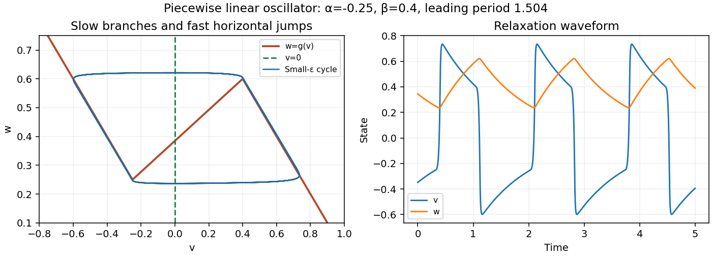
On the attracting right branch, the leading fast balance is $w=1-v$, so $\dot{w}=v=1-w$. On the left branch it is $w=-v$, so $\dot{w}=-w$. The slow travel times are thereforeBoth are positive because $w_R>w_L$. The fast jumps contribute vanishing time as $ϵ\to 0$, giving the piecewise linear relaxation-oscillator periodFor the illustrated $\alpha =-0.25$, $\beta =0.4$, the leading period is $1.5041$ in the given nondimensional time units.