Solutions to all three questions of the mathematical physiology course of the University of Oxford examination held on 31 May 2023. Original paper: public examination PDF, inclusive bundle pages 321–324; paper pages 1–4. All eighteen lettered parts are covered, including the third question even though only the best two answers counted. Question 1(c) contains a printed exponent error; Question 2(f) requires a signed recovery cutoff. Both are explained where they arise.
Write , and for the three concentrations. The letters denote chemical species; the forward arrow represents association of one molecule of each reactant into one complex, and the reverse arrow represents dissociation. The positive constants and are the respective reaction rate constants. For an elementary chemical reaction, the law of mass action gives forward and reverse reaction ratesEvery forward event removes one molecule of each reactant and adds one complex; a reverse event reverses those changes. Thus the reaction-rate equations areThe units of are inverse concentration per unit time, whereas has units of inverse time. Adding the equations gives the independent conservation lawsIn particular is constant, but this is a consequence of those two conservation laws. The total need not be constant: association changes the number of separate molecules.
For the general stoichiometry, take to be positive integers. The net reaction rate and stoichiometric vector areConsequentlyThe factors outside count molecules consumed per event; the powers inside express the law of mass action. The corresponding conservation laws are and . No factorial is required in this deterministic convention for the reaction rate constant.
There are four reversible transitions of the ion channel, each changing exactly one gate:These are first-order reaction-rate equations: their reaction rate constants are per-gate transition rates. In the continuous-time Markov chain interpretation, simultaneous changes of both gates have probability of order , so there is no direct diagonal transition in its infinitesimal generator matrix.
Normalize the total channel density to one. For independent permissive gates in an ion channel, the probability that the gate is open is , and the probability that the gate is open is . The joint probability is the product of the appropriate open or closed probabilities, givingIn particularThe original PDF really prints , rather than , on the final factor. That expression fails normalization of a probability distribution and does not give the closed- probability at ; the displayed correction is necessary. If are literal densities with conserved total density , multiply each expression by .
The product additionally assumes initially independent events and independent gate transitions. The transition scheme alone permits initially correlated gates and does not force this factorization at every time. The all-closed initial preparation used below satisfies the required product assumption.
For each state, add its incoming reaction rates and subtract its outgoing reaction rates. This gives the master equationSumming gives , verifying the conservation law for total channel density. Nonnegative initial densities stay nonnegative because every loss term vanishes when its own density reaches zero.
With total density one, the open probabilities for the individual gates are and . Adding the relevant master equations cancels transitions of the other gate:These marginal ordinary differential equations hold even for correlated initial gates. Their product gives when the independence assumption in part (c) holds. Solving the first-order linear differential equations from the all-closed initial state givesPut . ThenFor positive opening rates this increases strictly from zero, so its half-equilibrium time is uniquely determined by :If an opening rate is zero, the all-open equilibrium density is zero and a nontrivial half-rise time is undefined.
The two identical gates are independent Bernoulli random variables, so their open count has a binomial distribution. Multiplying by the independent factor gives the normalized channel densitiesExplicitly,The binomial coefficient counts which of the two distinguishable gates is open. At open count , the total -opening rate is and the total closing rate is . Dividing the expected value of that count by two therefore recovers the same single-gate ordinary differential equation:For the specified initial conditions and common rate sum , the all-open fraction isThus, assuming positive opening rates,Three gates take longer to reach half their final all-open fraction than two gates: all three activation factors must build up simultaneously.
In the Hodgkin-Huxley model, is the intracellular-minus-extracellular membrane potential, is the membrane capacitance per unit area, and is the applied inward electric current per unit area. A space clamp makes spatially uniform, leaving temporal ordinary differential equations. With outward ionic electric current positive, the capacitance balance is .
The variables lie between zero and one. They describe sodium activation, potassium activation and availability against sodium inactivation, respectively. Thus larger means less inactivation. Their voltage-dependent limiting values are , and are their positive relaxation time constants.
Each ionic term has the Ohm's law form conductance times driving potential. The sodium term has instantaneous electrical conductance , the potassium term has instantaneous electrical conductance , and the leak term has constant electrical conductance . Here the constants are maximal electrical conductances per area, and are the corresponding reversal potentials. The factors and arise from independent permissive gates in an ion channel. A conducting channel carries zero net ionic electric current at its reversal potential.
Use the three standard reduction assumptions: relaxes much faster than and can be replaced by ; the two slower gates have the same time constant, ; and their limiting open fractions have a voltage-independent sum, . The constant-sum assumption is essential: equality of two time constants by itself does not preserve a moving voltage-dependent sum.
For , addition of the two gate ordinary differential equations givesThe specified initial condition is . Uniqueness for this first-order linear differential equation gives , hence for all time. The remaining two ordinary differential equations areThese assumptions give a planar reduction of the Hodgkin-Huxley model. The FitzHugh-Nagumo model keeps its fast activation and slow recovery variable geometry, approximating the voltage response by a cubic polynomial and the recovery response by a linear function after nondimensionalization. The polynomial equations in part (c) are a further model simplification; they are not an exact algebraic consequence of arbitrary original gate functions.
Assume . At an equilibrium, , soThe nonzero roots areConsequently, with , there are three distinct equilibria for , two distinct equilibria for , and only the origin for . At equality the two nonzero equilibria coincide; for they both have . Geometrically, is the maximum of the concave quadratic .
Since , the Jacobian matrix at the origin isThus the origin is always asymptotically stable. Its eigenvalues areWriting , the origin is a stable node for and a stable focus for . At it is a degenerate node: the repeated negative eigenvalue has only one independent eigenvector, since the nonzero off-diagonal entry prevents being a scalar matrix. If , then and every permitted gives a stable focus. This change from node to focus does not change stability and is not a Hopf bifurcation.
Take and let with the other parameters fixed. The nullclines are the cubic polynomial graph and the line . In the phase plane, increases below the cubic polynomial graph and decreases above it; increases below the line and decreases above it. The fast ordinary differential equation, in time , freezes and gives .
At , the fast roots are . Their linear stability follows from , and . Thus a fixed falls towards the resting branch, whereas a fixed rises towards . If , the first fast segment instead settles down towards , followed by the same recovery excursion. The threshold is the leading singular perturbation threshold; finite- corrections matter for initial values approaching with .
LetThese are the roots of . The outer branches and of the critical manifold are attracting under fast motion; the middle branch is repelling. The full excursion has four stages.
- Fast activation: nearly horizontal movement towards , on the time scale, apart from the usual matching tails.
- First slow phase: motion along from down to . Here rises and slowly falls, because on the positive outer branch. This takes order-one time for fixed .
- Fast repolarization: near the right fold point of a critical manifold, the attracting branch ends. With nearly constant, drops to the negative root of . The jump takes the fast time scale; a thin neighborhood of the fold has an intermediate fold delay.
- Second slow phase: motion along the negative attracting branch from towards from below, while falls towards zero. This is the refractory recovery and has order-one duration to a fixed small cutoff; exact return to the equilibrium takes infinite time.
For this cubic polynomial, the landing point is explicit. Since , comparison of the quadratic coefficients givesThus a graph of has a rapid rise, a slowly falling elevated plateau, a rapid fall through zero to a negative undershoot, and a slow approach back to zero. The figure shows both the phase plane and a computed time trace. The smaller initial perturbation stays near the resting branch and produces no elevated plateau.
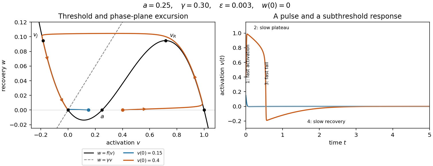
The four-stage description concerns the singular limit. Close to a simple fold point of a critical manifold, balancing the local quadratic activation term with the slow drift gives and for fixed parameters. These layers shrink compared with the slow phases and do not alter the leading time integrals below.
On an attracting branch of the critical manifold, to leading order. The chain rule therefore givesThe initial fast segment ends at , and the first slow phase ends at the right fold point of a critical manifold, . HenceOn this interval and . The integrand is negative, but the upper limit is smaller than the lower limit, so . The numerator tends to zero at the fold while the denominator remains positive; the leading integral is finite. Fast segments and the fold delay give vanishing corrections as .
The requested second phase is the second slow recovery phase, beginning after the downward fast jump. Its starting point is , fixed by , with the negative root chosen. Along it the same chain rule givesThe approach is to zero from below. Thus, if the printed cutoff is a signed value, it must satisfy and . If denotes a small positive magnitude, the endpoint is instead . To express both conventions unambiguously, put and writeThere is no positive small endpoint on this leading slow branch. A positive cutoff would require a different event or finite- oscillatory recovery.
For bounded negative and ,Integration therefore gives the useful more detailed approximationTaking also , the leading logarithm isIndeed near zero, and the slow equation is , so at fixed the exact leading logarithmic coefficient is . Its large- limit is , agreeing with the integral.
The order of approximation matters: first take the singular limit at fixed , then the large- and small-cutoff limits. For simultaneous limits, a sufficient separation near rest is . Otherwise the fast and recovery time scales merge, and these slow-branch formulas need not describe the late-time motion.
In this two-pool calcium model, is the cytosolic calcium ion concentration, and measures calcium in an intracellular store, such as the endoplasmic reticulum. The variables in these balances are expressed using compatible effective volumes, so internal transfers enter their two equations with equal and opposite signs. If actual compartment concentrations use different reference volumes, the corresponding volume ratio must first be included in their balances.
The flux pumps calcium from the cytosol into the store, releases it back, and is passive store leakage back to the cytosol. The external input supplies cytosolic calcium, while exports it from the biological cell. Thus have units of inverse time and all five fluxes have units of concentration per time. Their directions can be sketched asAdding the two ordinary differential equations verifies the total calcium balanceInternal uptake, release and leakage redistribute calcium; only the exchanges across the cell membrane change this total. In particular any equilibrium must have when .
Choose positive reference concentrations and a reference flux , and defineOverdots now mean derivatives with respect to the dimensionless time . The store balance becomesThe total balance becomes . ThereforeandThe reference quantities are scale choices, not additional kinetic variables; typically the response functions supply natural saturation concentrations and a maximal uptake flux. The identity checks the nondimensionalization. A small means store exchange is fast compared with external cytosolic removal.
At any equilibrium, the first balance gives and the second gives . For every fixed ,andThe intermediate value theorem and strict monotonicity give precisely one positive root for each . Since , the implicit function theorem makes this a smooth nullcline. For every , therefore,is the unique positive equilibrium. Graphically, draw the vertical line through the given graph: it meets the graph once, even on its steep descending section. This vertical line is the condition for simultaneous stationarity; the full nullcline at finite is actually .
Eliminate from the first equation before linearization:All partial derivatives below are evaluated at . The Jacobian matrix isIts trace and determinant areBy linear stability of a planar equilibrium, a positive trace makes both real eigenvalues positive or gives a complex pair with positive real part. The equilibrium is consequently unstable precisely whenA negative trace gives asymptotic stability; equality leaves a purely imaginary pair and requires a separate nonlinear bifurcation calculation. In particular, the unique positive equilibrium is never a saddle equilibrium.
Differentiate the identity using the chain rule:Substitution into the trace givesBecause , the exact instability condition isFor fixed and fixed equilibrium location, the correction tends to zero with . To leading order this isThus instability requires the descending nullcline to be steeper than a line of slope . The sign of the finite- correction makes the exact unstable interval slightly smaller. Since can make small, the approximation quantitatively requires at the point in question; merely comparing with one can be insufficient.
On the descending part of the graph, mark the two tangency points whereChoose the crossings that enclose the portion with . For fixed strictly between these values and sufficiently small , the unique equilibrium is a repelling equilibrium by part (e). The endpoints here are leading singular limit values; at finite the boundaries instead solve and approach these tangencies when the crossings are nondegenerate.
There is a necessary qualification: such an interval exists only when is large enough that the descending graph actually attains slopes below . If , one needs . The supplied graph has a very steep descending section, but an arbitrarily small positive need not satisfy this condition. For , numerical evaluation gives , so the leading threshold is . A graph alone does not remove this parameter restriction.
The fast motion is especially informative. In fast time ,At leading order is constant, so fast paths are straight lines with slope . Along such a line, the fast eigenvalue at the nullcline isIt is negative on the two outer attracting segments and positive on the intervening repelling segment. The tangencies defining are consequently the fold points of a critical manifold when it is expressed in the coordinates . They are not generally the maximum and minimum of itself.
For , slow motion on an attracting segment followsOn the left attracting segment this moves towards increasing ; on the right attracting segment it moves towards decreasing . Each segment ends at a tangency and is followed by a fast jump along a line of slope to the other attracting segment. This constructs the limiting relaxation oscillation. The figure uses , for which and ; the marked endpoints change with .
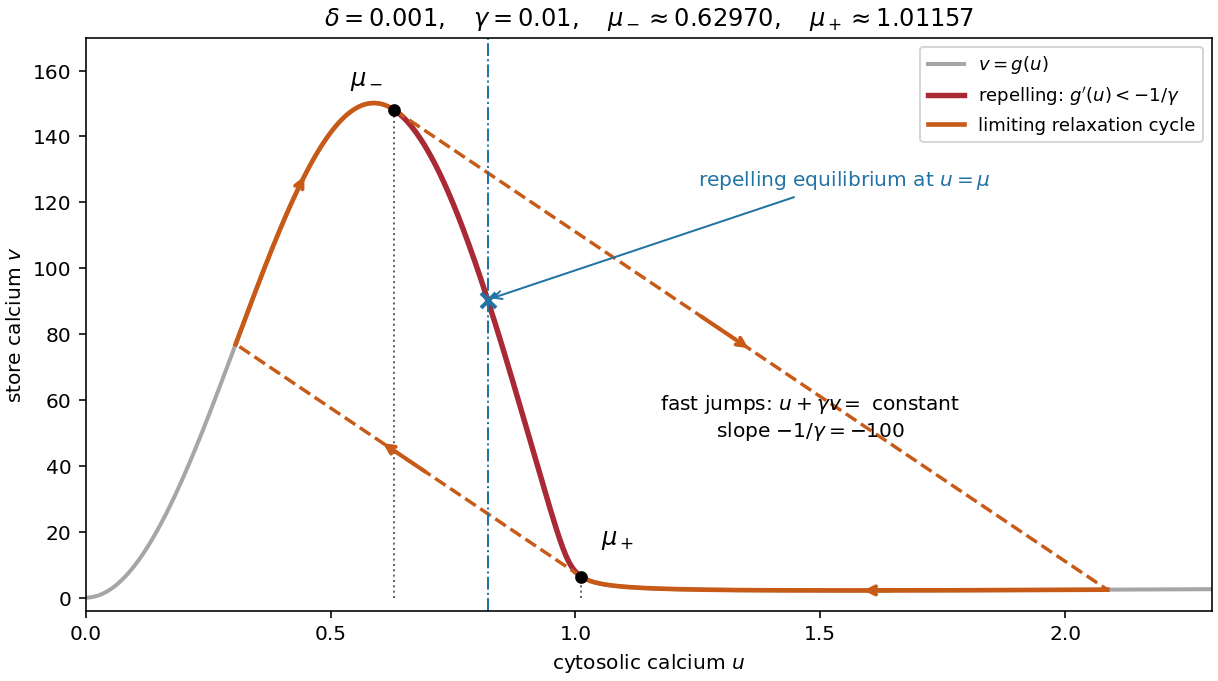
To justify existence of a periodic orbit of the full planar system, rather than just draw a formal cycle, first establish a compact trapping region. The positive quadrant is forward invariant: at , , and at , . MoreoverChoose above the initial store value. Since when ,Thus the rectangle , is a positively invariant set if and the initial point lies inside it. Every forward solution is bounded. There are no equilibria on its axes for , and its sole interior equilibrium is a hyperbolic equilibrium point with both eigenvalues having positive real parts in the strict unstable range. A sufficiently small neighborhood of this repelling equilibrium has outward flow; deleting it leaves a compact trapping region with no equilibria. The Poincaré-Bendixson theorem then supplies a periodic orbit.
Hence periodic solutions exist throughout the strict unstable interval, interpreted with the finite- correction above. This argument establishes existence, without asserting uniqueness, the criticality of possible endpoint Hopf bifurcations, or absence of coexisting periodic orbits outside the interval.
In the Hodgkin-Huxley model, is the membrane potential, the voltage inside the axon relative to outside. The space clamp assumption makes it spatially uniform. The gating variables lie between zero and one: describes sodium activation, describes availability against sodium inactivation, and describes potassium activation. Thus large means channels remain available, not that inactivation is strong.
The left side is capacitive electric current per unit membrane area. The imposed is inward-positive applied electric current. The other terms are outward-positive ionic electric currents: sodium with electrical conductance , potassium with conductance , and a passive leak with conductance . Each current is its conductance times the difference between and the corresponding reversal potential , or . The coefficients are maximal conductances; the gate factors represent independent permissive gates in an ion channel.
For each gate, is the equilibrium opening/availability fraction at fixed voltage and its exponential relaxation time. The equation follows from two-state ion-channel gating: if , thenVoltage feedback couples these otherwise elementary gating equations to the membrane potential and produces action potentials.
Write . In the physically relevant strip , , the zero-current nullcline satisfiesThe left side increases strictly from zero to infinity, so there is exactly one nullcline height for each interior voltage. If is positive at the endpoints, its curve joins to ; when low-voltage activation is idealized as exactly zero, the limiting left branch can lie on .
The signs of the derivatives explain its folds:At low voltage, potassium's approximately linear contribution dominates and . During rapid sodium activation the last negative term can dominate, giving . Once activation saturates, becomes small and again. This folded conductance-model nullcline has the familiar shape: the curve has descending outer branches and an ascending middle branch in the plane. Equivalently, an intermediate fixed can give three zeros of as voltage rises, with positive, negative and positive at those crossings.
The rapid-activation description permits this folded shape; exact fold positions depend on . The figure supplies an explicit admissible sigmoid example. Its right panel shows as well as the recovery nullcline and an oscillating trajectory.
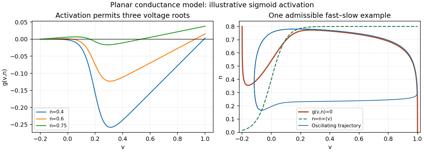
The voltage nullcline is and the recovery nullcline is . In the relevant region , so below the voltage curve and above it . Below the recovery curve , while above it .
For small , the outer voltage branches with attract fast voltage motion; the middle branch with repels it. Arrange the intersections so the equilibrium is on that middle branch, with recovery increasing along the high-voltage attracting branch and decreasing along the low-voltage attracting branch. The trajectory then drifts towards a fold, jumps rapidly to the other attracting branch at nearly constant , and repeats. This is a relaxation oscillation.
The local linear stability calculation supports the construction. At an equilibrium,A sufficiently steep recovery curve gives positive determinant, while gives positive trace. Hence the equilibrium is a repeller. The bounded physical rectangle can be chosen forward invariant, and a small neighborhood of the repeller removed to give a trapping annulus. The Poincaré-Bendixson theorem then supplies a periodic orbit. These conditions can be realized because the recovery function and the applied current control the intersection and its slope; oscillation is possible, not forced for every choice.
For the illustration, , , , , , and . The rectangle has inward-pointing flow, and the displayed numerical trajectory realizes the folded-branch mechanism.
The nullclines are and . The two outer pieces of have slope ; the middle piece has positive slopeThe curve is continuous, with folds and . The unique equilibrium is . Its Jacobian matrix has trace and determinant , so it is unstable. The outer branches attract the fast voltage motion.
The jumps are almost horizontal in the phase plane, because changes negligibly on the fast time. Below , voltage increases; above it, voltage decreases; increases on the right of and decreases on the left. These signs provide a closed trapping region around the indicated route for sufficiently small positive , with the unstable equilibrium excluded, giving a periodic orbit by the planar return-map or Poincaré-Bendixson theorem argument. The continuous piecewise linear field is locally Lipschitz, so solution uniqueness is available at the corners.
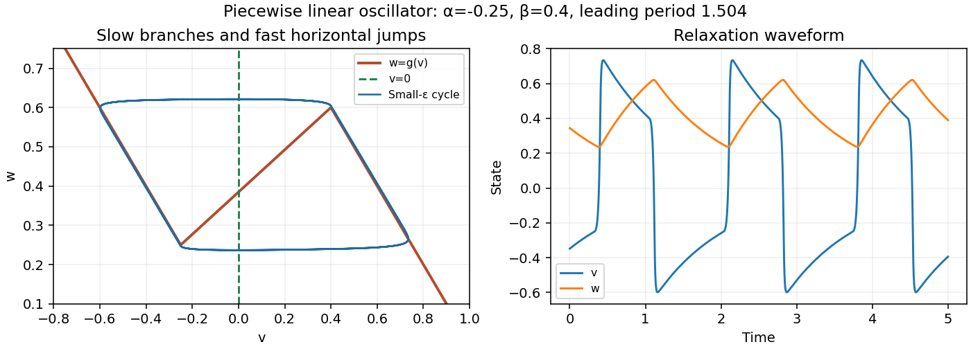


On the attracting right branch, the leading fast balance is , so . On the left branch it is , so . The slow travel times are thereforeBoth are positive because . The fast jumps contribute vanishing time as , giving the piecewise linear relaxation-oscillator periodFor the illustrated , , the leading period is in the given nondimensional time units.
Let be pressures in the arterial reservoir, venous reservoir and left ventricle. Constant vascular compliances relate volume changes to pressure changes. The ventricular elastance relation iswhere is the unstressed ventricular volume and is the time-dependent inverse compliance. Define the positive part . The systemic, aortic-valve and mitral-valve flows areEach is a positive hydraulic resistance. The aortic valve permits outflow only when ventricular pressure exceeds arterial pressure, and the mitral valve permits filling only when venous pressure exceeds ventricular pressure.
Mass conservation, with blood treated as incompressible, givesSubstitution and multiplication of the first two equations by give exactlyAdding the three original balances gives zero total volume change. This is a three-compartment ventricular circulation model.
During isovolumetric contraction, ventricular pressure lies between the venous and arterial pressures, . Both valves are closed, so and ventricular volume remains at its end-filling value . ConsequentlyHere is end-diastolic ventricular volume and is the zero-pressure/unstressed volume.
The arterial and venous reservoirs still exchange systemic blood:If contraction is short compared with both and , the fractional changes are small andwhere the superscript values refer to the beginning of contraction. Thus pressure can rise rapidly in the left ventricle through increasing elastance while the other pressures are approximately fixed. This stage ends when reaches and the aortic valve opens.
During ejection the mitral valve is closed, so . Adding the arterial and ventricular balances cancels aortic flow:where the last approximation assumes .
Model the rapid contraction as a switch to approximately constant systolic elastance , with the systolic ventricular compliance. A sufficiently small aortic-valve resistance makes after a short pressure-equalization transient. The systolic pressure must be high enough to open the valve, . During that transient neglect systemic runoff. Conservation of combined arterial and stressed ventricular volume givessoThis is an approximation across a rapid transient, not a discontinuity at finite valve resistance. The subsequent common pressure obeys , givingThe source's in this expression denotes the same systemic resistance .
At the end of firing, the remaining ventricular volume is . The stroke volume is , henceThe assumptions are a closed mitral valve throughout ejection, negligible venous pressure, rapid valve equalization relative to systemic runoff, and nearly constant systolic elastance during the interval measured by . These give the ventricular ejection pressure and stroke-volume approximation.
For a constant solution , its delayed value is also . The equation becomes , so the only constant equilibria are . The delay differential equation requires the same constant history to realize each equilibrium.
A positive solution stays positive, sinceTherefore the sign of is exactly the sign of . Initially the given history below one makes . If crosses one upwards at time , it continues growing until , because the feedback still sees earlier values below one. It reaches a maximum when the delayed value crosses one. Similarly, after a downward crossing at , it continues decreasing until and reaches a minimum then.
This delayed reversal makes overshoots and undershoots possible. In a derivative sketch, positive lobes persist until one delay after upward crossings, followed by negative lobes persisting until one delay after downward crossings. Sustained oscillation depends on the delay; a short delay can instead give convergence to one. The example shown has and a history identically .
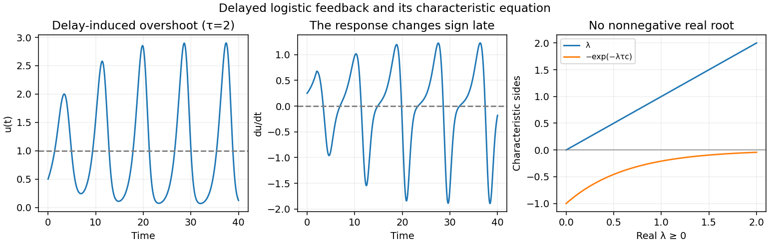
Overshoot, delayed derivative sign changes, and the absence of a nonnegative real characteristic root
. Details. 
Put . Then , so the linearization is . A mode gives the characteristic equation of a delay differential equationFor real , the left side is nonnegative and the right side negative. The two real graphs therefore never meet there, as drawn in the figure. There is no nonoscillatory exponential instability. If stability is lost, the unstable eigenvalues must be a nonreal conjugate pair, producing oscillatory growth; absence of a positive real root alone does not imply stability.
For a purely imaginary root with , separating real and imaginary parts givesThus and , . The first crossing isFor there is no root with nonnegative real part. Indeed, write with . The real equation forces , hence . But the imaginary equation gives , contradicting .
Differentiate the characteristic equation along the root:The imaginary roots are simple because , and they cross into the unstable half-plane as delay increases.
One can also check the nonlinear Hopf bifurcation directly. With and small amplitude , substituteThe constant and second harmonics at order give the displayed coefficients. Put . At order , absence of resonant first harmonics requires and . HenceThe nonzero coefficient verifies a branch of small periodic solutions for , consistent with the transverse Hopf bifurcation in the delayed logistic equation. This is the delayed logistic Hopf threshold.
At the crossing the angular frequency is , so the limiting small-amplitude period isThis is the period of the bifurcating infinitesimal oscillation. Finite-amplitude oscillations away from the threshold need not have period exactly .
Articles by others on the same topic
There are currently no matching articles.