Past exam of the mathematics course of the University of Cambridge / 2001 / iii / Paper 33 (Time Series and Monte Carlo Inference)

Write $C={\int }_{\mathbb{R}}f(x)dx$, so $0<C<\infty$. The finite envelope condition means that $f\le Mg$ almost everywhere; in particular, the proposal must cover the support of the target.

For each independent proposal $Y\sim g$, generate an independent $U\sim \mathrm{Unif}(0,1)$ and accept $Y$ precisely whenDiscard a rejected proposal and continue. The ratio is in $[0,1]$ and is needed only where $g(Y)>0$. Neither evaluation of $C$ nor prior knowledge of the normalized target is required.

To prove the output law, for any measurable set $D$ the joint probability of acceptance and a proposal in $D$ isDividing by the total acceptance probability $C/M$ gives ${\int }_{D}f(y)/Cdy$, the target probability. Independent proposal-uniform pairs give independent accepted observations. With a finite proposal list there can be no accepted value; with continued independent trials, acceptance eventually occurs almost surely because $C/M>0$.

The acceptance mass for an unnormalized rejection envelope follows by integrating the proposal-specific acceptance probability:The inequality $f\le Mg$ also gives $C\le M$, so this is a valid probability. It is the same at every independent trial.

If $J_i$ indicates acceptance of the $i$th proposal, then $J_1,\dots ,J_n$ are independent Bernoulli distribution variables with parameter $C/M$. Hence the accepted count $K={\sum }_i{J}_i$ satisfiesIts variance is $n{p}_{\mathrm{acc}}(1-p_{\mathrm{acc}})$. Conditional on any acceptance pattern, the accepted values have independent target probability density function $h$; mixing over patterns retains this product law conditional on their count.

For normal rejection sampling with an exponential envelope, complete the square in the probability density function ratio:The maximum occurs at $x=\lambda$, which lies in the support because $\lambda >0$. ThusThe PDF exponent is $e^{{\lambda }^2}$ inside the square root; this distinction is lost in the converted TeX.

The acceptance rule simplifies toAn exponential proposal can be generated as $Y=-{\lambda }^{-1}\log V$ from an independent uniform distribution value $V$. Since the target is normalized, the overall acceptance probability is $1/M(\lambda )$. To maximize it,Therefore the optimal rate is $\lambda =1$, with acceptance probability $\sqrt{\pi /(2e)}$.

Finally, give each accepted half-normal distribution value $Y$ an independent fair sign $R\in \{-1,1\}$ and output $Z=RY$. On each half-line its probability density function is half the reflected half-normal distribution probability density function:Consequently $Z\sim N(0,1)$. The sign must be drawn independently; rejection itself does not supply it.

For the Metropolis–Hastings algorithm, start at a point $x$ with positive target probability density function. Draw $Y$ from a proposal probability density function $q(y\mid x)$, generate an independent uniform distribution value $U$, and set the next state to $Y$ ifOtherwise retain $x$, including that repeated state in the sample. Where a proposed forward move is possible but its reverse probability density function vanishes, its acceptance probability is zero. Unknown normalizing constants in $\pi$ cancel.

For distinct states, the accepted probability flow iswhich is symmetric in $x,y$. This detailed balance identity, together with the holding probability, proves that $\pi$ is invariant. Under appropriate irreducibility and aperiodicity conditions the chain converges to $\pi$; successive states are generally dependent.

The Gibbs sampler updates coordinates from their full conditional distributions. In a systematic sweep, draw successivelyEach update preserves the target joint law: integrating the old coordinate against its conditional probability density function and replacing it by an independent draw from that same conditional leaves the joint probability density function unchanged. The composition of the coordinate updates therefore also preserves $\pi$. A Gibbs sampler coordinate move can be regarded as a Metropolis–Hastings algorithm move with acceptance probability one. Systematic sweeps preserve stationarity but need not themselves be reversible. Initialization away from stationarity requires convergence before treating the draws as approximately target-distributed, and dependence must be accounted for in Monte Carlo method error estimates.

Assume ${\sigma }_1,{\sigma }_2>0$ and $|\rho |<1$, as required for the displayed nonsingular probability density function. Put $z_j=(x_j-{\mu }_j)/{\sigma }_j$. Its quadratic exponent isHolding $x_2$ fixed and normalizing the term depending on $x_1$ givesThe analogous completion of the square gives

Using independent draws ${\eta }_{1,r},{\eta }_{2,r}$ from the standard normal distribution, a sweep isUse the newly drawn first coordinate in the second update. Recording the pairs after each sweep gives the dependent sample.

The Gaussian Gibbs sweep autocorrelation makes the dependence explicit. In standardized coordinates, substitution yieldsThe new noise has variance $1-{\rho }^4$, so the stationary variance is one and the lag-$h$ sweep autocorrelation is ${\rho }^{2h}$. Thus the sampler converges geometrically for $|\rho |<1$, but becomes slow near perfect correlation. When $\rho =0$, complete sweeps yield independent pairs. The singular cases $|\rho |=1$ do not have the stipulated two-dimensional probability density function.

Here the proposal is $Y=x+\eta$ with $\eta \sim N_2(0,I_2)$. Its probability density function depends only on $\Vert y-x{\Vert }^2$, so $q(y\mid x)=q(x\mid y)$. The determinant and normalizing constant of the target also cancel. With $Q$ as in the preceding entry,Equivalently, writing $u_j=(y_j-{\mu }_j)/{\sigma }_j$ and $z_j=(x_j-{\mu }_j)/{\sigma }_j$,One can also compute the exponent without subtracting two large quadratic forms:Generate two independent standard normal distribution proposal increments, compute this log ratio, and accept when $\log U\le \min (0,\log (\pi (Y)/\pi (x)))$. Retain the previous pair on rejection. Detailed balance gives the correct invariant distribution, and the everywhere-positive Gaussian proposal makes this random-walk Metropolis algorithm chain irreducible; a rejection probability provides a holding step. The resulting target-distributed pairs are dependent, with proposal scale and target anisotropy controlling how quickly they mix.

Write ${\sigma }_{\epsilon }^2$ for the driving white noise variance and $\Theta (z)=1+{\sum }_{\ell =1}^q{\theta }_{\ell }{z}^{\ell }$. The autoregressive polynomial factors asThe discrete Gaussian white noise values are independent. The roots of $\Phi$ are outside the unit disc, so expanding $\Theta (z)/\Phi (z)$ gives an absolutely summable causal time-series representation. Hence $x_t$ is a centered Gaussian process formed from driving white noise values at times at most $t$. In particular, for $k>q$, every driving white noise value ${\epsilon }_{t-\ell }$ with $\ell \le q$ is independent of $x_{t-k}$. The autocovariance tail recurrence of a causal ARMA process follows by taking covariance of the recursion with $x_{t-k}$:

The roots of the characteristic polynomial of this tail recurrence are $1/2$ and $1/3$. Let $k_0=\max (q-1,0)$. There exist constants $c,d$ such thatFor example, put $a=6{\gamma }_{k_0+1}-2{\gamma }_{k_0}$ and $b=3{\gamma }_{k_0}-6{\gamma }_{k_0+1}$; then $c=2^{k_0}a$ and $d=3^{k_0}b$ reproduce the two starting values and therefore the whole recurrence. Choose $C$ strictly larger than $|c|+|d|$ and all the finitely many values $2^k|{\gamma }_k|$ with $0\le k<k_0$. Symmetry ${\gamma }_{-k}={\gamma }_k$ now givesFor negative $k$ this is stronger than the requested bound with $2^{-k}$. It also proves ${\sum }_{k\ge 1}k|{\gamma }_k|<\infty$.

For the Fourier calculation, take $D=2m+1$ positive and $T=DN$ positive. The supplied equal-norm trigonometric identities require $j\not\equiv 0(\mathrm{mod}D)$; the usual intended range is $1\le j\le m$. Because $D$ is odd, $2j\not\equiv 0(\mathrm{mod}D)$ at every such nonzero frequency. The geometric series of $e^{i\omega t}$ and $e^{2i\omega t}$ over $T$ terms vanish. They implyOther integer values of $j$ reduce modulo $D$; folding a negative frequency changes the sine coefficient only by a sign. The permitted zero frequency is handled below.

Grouping the double expectation sum according to the time lag yieldsReplace the two truncated sums for lag $k$ by full sums. Their total isEach replacement adds at most $k$ terms, each of absolute value at most one. This gives the finite-record Fourier covariance bound:Both coefficients have expected value zero, so this expectation is their covariance.

For each finite $T$, $(A,B)$ has a multivariate normal distribution because it is a linear transformation of the Gaussian observation vector. If the variances converge to $v_A,v_B$, its characteristic function converges tosince the cross-covariance tends to zero. This is the characteristic function of two independent centered normal variables; zero limiting variances are allowed.

We can calculate the variance limits rather than merely assume their existence. Grouping the cosine covariance sum givesOver a full record, ${\sum }_{t=1}^T{c}_t{c}_{t+k}=(T/2)\cos (\omega k)$. Truncation changes this by at most $k$. The same statements hold for the sine products. Consequentlyand the identical main term and bound apply to $\mathbb{E}{B}^2$. Absolute summability now gives

Specify the spectral convention to identify this limit. LetHere $f_2$ is the two-sided probability density function on $[-\pi ,\pi ]$, and $s$ is the one-sided probability density function on $[0,\pi ]$, satisfying ${\gamma }_k={\int }_0^{\pi }s(\omega )\cos (k\omega )d\omega$. Thus each variance limit is $f_2(\omega )=s(\omega )/2$. For this particular model, the filter representation also gives

For the specified squared-sum estimator, an exact expectation calculation uses $c_t{c}_u+s_t{s}_u=\cos (\omega (t-u))$:The missing tail and the $k/T$ terms vanish; indeed the bias is $O(T^{-1})$ by the exponential covariance bound. Therefore $I(\omega )$ is asymptotically unbiased for the one-sided probability density function $s(\omega )$. Under the common two-sided convention its limit in expectation is $2f_2(\omega )$, so $I(\omega )/2$ is the appropriately normalized estimator.

At an interior frequency with $s(\omega )>0$, the joint Gaussian limit gives the exponential limit of a one-sided periodogram:Moreover, for a centered Gaussian pair,The nondegenerate exponential limiting law rules out convergence in probability to $s(\omega )$. Thus the unsmoothed periodogram is not consistent at frequencies with positive spectrum, despite its asymptotic unbiasedness. If $s(\omega )=0$, the nonnegative estimator has expectation tending to zero and is consistent there by Markov's inequality. Smoothing an increasing number of nearby ordinates while shrinking the frequency bandwidth can remove the positive-spectrum variance obstruction.

For $j\equiv 0(\mathrm{mod}D)$, the sine coefficient is identically zero and the cosine coefficient is the normalized sum of the observations. The corrected limits areThe joint limit is $(N(0,s(0)),0)$, independent in the degenerate sense. The exact expectation formula for $I$ still applies and tends to $s(0)$, but now $I(0)/s(0)\stackrel{d}{\to }{\chi }_1^2$ when $s(0)>0$, with limiting variance $2s(0{)}^2$. The estimator is again inconsistent. This covers the zero frequency allowed by the printed inequality on $j$.

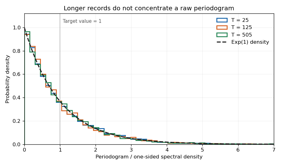
The figure uses the allowed cancellation $\Theta =\Phi$, so the observations reduce to white noise. Orthogonal Fourier projections give the exponential law exactly at each plotted record length; increasing the record does not narrow the individual periodogram ordinate.

For the three-coordinate state realization of an ARMA(1,1) process, the observation row and transition matrix areThe first row of $G{S}_{t-1}$ is $x_{t-1}$ by the previous-time recursion; the second row is zero until the new white noise value is added; and the third row copies ${\epsilon }_{t-1}$. Hence the state equation has noise covariance

We use the causal state model, in which the new driving noise is independent of the previous state. The Gaussian filtering with exact observations form of the Kalman filter alternates prediction through the state equation with conditioning on the next observation. Given the posterior expected value and covariance at time $t-1$, independence of the new white noise value gives predictive expected value $a_t=G{\hat{S}}_{t-1}$ and predictive covarianceProject through the observation row to getThe residual $v_t=x_t-{\hat{x}}_t$ is the innovation. Conditioning the joint Gaussian state-observation vector adjusts the expected value according to this residual and reduces the covariance. In this exact-observation model, the updates can be writtenThus $F{\hat{S}}_t=x_t$ and $F{P}_t{F}^{\top }=0$: the observed linear combination of the state is now known exactly, though other state combinations remain uncertain.

The PDF's stated prediction variance omits $FQ{F}^{\top }={\sigma }^2$. This omission cannot be used in a valid likelihood: for the AR(1) specialization below it would give zero prediction variance after the first observation. The required likelihood calculation uses the corrected innovation variance just derived.

For stationary initialization of an ARMA(1,1) state with $|\varphi |<1$, take ${\hat{S}}_0=0$ and the unconditional stationary covariance. The causal coefficients are $1$ at lag zero and $(\varphi +\theta ){\varphi }^{j-1}$ at lags $j\ge 1$, givingSince $S_0=(x_{-1},{\epsilon }_0,{\epsilon }_{-1}{)}^{\top }$, the cross-covariance with ${\epsilon }_0$ is zero and that with ${\epsilon }_{-1}$ is ${\sigma }^2$. ThereforeDirect substitution verifies $P_0=G{P}_0{G}^{\top }+Q$. If prior state information is available, instead use its conditional expected value and covariance. A diffuse initialization is another option when the initial state is genuinely unknown, but it changes the finite-sample likelihood and should not silently replace the stationary initial law.

By the Gaussian prediction step,The chain rule for probabilities for the joint probability density function therefore givesTaking minus twice its logarithm shows that maximum likelihood estimation is equivalent to minimizingwith each $V_t$ and ${\hat{x}}_t$ evaluated at the candidate parameters and the specified initialization. The corrected $+{\sigma }^2$ is essential in every $V_t$.

For the stationary causal AR(1) case, $\theta =0$ and $|\varphi |<1$. The first observation is $N(0,{\sigma }^2/(1-{\varphi }^2))$, whereas each later conditional observation is $\varphi x_{t-1}+{\epsilon }_t$. HenceThis also gives a direct counterexample to the uncorrected PDF variance: with $\theta =0$, $FG=\varphi F$ and $F{P}_{t-1}{F}^{\top }=0$ after observing $x_{t-1}$, so its printed expression would give $V_t=0$ for $t\ge 2$.

To compare the conditional and stationary AR1 likelihood estimators, putThen its negative twice log-likelihood isFor fixed $\varphi$, $\widehat{{\sigma }^2}=Q_T(\varphi )/T$. Writingthe exact interior score equation isThe stationary initial contribution is order one for a fixed interior parameter, while $C_T$ is order $T$. Discarding this lower-order contribution givesConditioning on $x_1$ makes this ratio the exact unconstrained conditional maximum likelihood estimate. Under the stationary initial law it is only the leading approximation: at an interior optimum,This approximation presumes a nondegenerate sample denominator and a true coefficient fixed away from the unit-root boundary; a finite-sample constrained optimum must respect $|\varphi |<1$.