Let , assumed finite. The displacement is . By stationarity, its two-time covariance is , with even for a real scalar process. Integrating over the two triangles of the square gives the Taylor turbulent dispersion identityA sufficient condition for ordinary long-time variance growth is with . The dominated convergence theorem then givesMore generally the necessary asymptotic condition for a finite positive variance-based diffusion coefficient is convergence of to that coefficient. Absolute integrability is sufficient, not necessary. A zero integral does not give nondegenerate ordinary diffusion. Moreover a second-moment calculation alone does not establish a normal distribution or an entire diffusive scaling limit; those require additional probabilistic assumptions.
For the specified positive autocorrelation, direct integration gives, when ,Thus the power-law velocity-correlation dispersion has the following regimes. If , the Lagrangian integral time is and ordinary variance growth holds, with . At the exact expression is . If ,For ,The last two regimes spread faster than ordinary diffusion and have no finite long-time diffusion coefficient. Their slowly decaying velocity memory is responsible. At short times all these correlations instead give the ballistic law .
Take and initially . Write , and set , . The advection-diffusion equation is . Integration by parts in the unbounded coordinate gives the longitudinal moment hierarchy for shear transportAll three moments obey Neumann boundary conditions at the walls. The initial values are , , . These manipulations require finite moments and vanishing boundary terms at ; diffusion of the compact initial distribution supplies the required decay for positive time.
The zeroth moment remains exactly . Since is a Neumann eigenfunction, put . Then and , givingFor the second moment, . Thus , withThe equation for has positive damping and bounded forcing, so remains bounded. In the equation for , the decaying term in contributes only a bounded accumulated transient. Over a complete nonzero-frequency cycle, and . ConsequentlyThis proves oscillating shear dispersion in an insulating channel, including the local-in- leading term, not just a cross-channel average. The instantaneous derivative retains bounded periodic oscillations; its cycle-averaged slope is . Thus is the leading second moment, rather than a literal rate proportional to .
The asymptotic statement holds for fixed positive diffusivity and fixed nonzero frequency, after times long compared with and the oscillation period. If , transverse diffusion adjusts rapidly to the changing shear flow, andThis is the cycle average of the instantaneous steady-shear enhancement . At exactly , there is no cycle average: and . Hence the zero-frequency and long-time limits do not commute. In the intermediate range , the shear is approximately steady at its initial amplitude and that latter enhancement is appropriate.
Write . The deformation gradient of one interval of shear flow is . An initial unit material line at angle therefore becomes . Its orientation, including the correct quadrant, isFor an unoriented line the angle is taken modulo . If , there is no shear flow: every and . The fluctuation and maximizing calculations below concern nonzero shear.
To quantify the renovating shear flow, use the intended isotropic model: each shear orientation is independent and uniform modulo . Independence by itself does not specify a probability law and cannot fix the answer. Under the uniform law, conditional on every earlier deformation, the relative angle to the next shear is again uniform. Thus the logarithmic increments are independent and identically distributed, even though the absolute orientation of the stretched material line need not be uniform. Since , only the one-step angular mean is needed.
Write , where , and . The supplied angular logarithmic integral, with parameter , givesTherefore the mean logarithmic stretching rate isThis is the mean logarithmic stretching in an isotropic renovating shear, and the strong law of large numbers gives the same almost-sure Lyapunov exponent. Taking without loss for this statistic puts it in the requested form .
For , . At small , ; at large , , tending to zero when increases at fixed shear rate. The maximizing nonzero solvesThe difference rises from zero up to and then strictly decreases to , so there is exactly one root beyond . Numerically,Very rapid renovation gives little deformation per interval and cancels the first-order mean stretch. Long intervals provide strong deformation but progressively align a material line with the shear direction, so one interval stretches it only algebraically in . Intermediate persistence combines substantial deformation with frequent reorientation, producing the finite maximum.
For the distribution, let , so the singular stretches of are . In the right-singular-vector basis, . Put . Factoring this expression and expanding its logarithm givesThe variance follows from angular orthogonality. These bounded independent increments implyAccordingly the central part of the large- stretch distribution is approximately described by a log-normal distribution, with density . This central limit theorem is not an assertion about arbitrarily extreme tails: the exact stretch has support inside .
For , the log-stretch fluctuations in an isotropic renovating shear haveTo leading order the mean and variance of both equal . Typical stretch is , while its mean grows as . These moment statements can be justified directly rather than extrapolating the central Gaussian approximation: expansion of givesfor fixed . In particular exactly. The leading small- log-normal approximation is especially precise in the many-small-renovations scaling with fixed and .
If the orientation law is not isotropic these formulas need not hold. For example, repeating a fixed shear direction gives , only algebraic stretch, and zero asymptotic logarithmic rate. The associated degenerate direction variables are independent, illustrating why the stated independence condition alone is insufficient to select the isotropic result.
The unperturbed sinusoidal cellular flow hasIts stream function is a first integral, so each trajectory lies on a level set of . This planar autonomous Hamiltonian flow has one degree of freedom and its conserved quantity reduces motion on regular levels to a quadrature: this is its integrability. The central cell has closed streamlines; the zero level is the grid of separatrices.
Solving both components of gives saddle equilibria at and center equilibria at . In the specified open square, the saddles are and the only interior center is . Centers at the outer square's corners are on its excluded boundary.
At a saddle the Jacobian matrix is with . If is even, the horizontal branches are unstable and vertical branches stable; if it is odd, those roles reverse. The branches extend along and and connect neighboring saddles as heteroclinic orbits. For example the bottom boundary flows from to , the right boundary from to , the top boundary from to , and the left boundary returns to . A connecting branch is unstable relative to its departing saddle and stable relative to its arriving saddle.
At a center the Jacobian matrix is , where now . Its eigenvalues are . The local definite extremum of surrounds it by closed streamlines, giving a neutrally stable center, not an attracting equilibrium. Central circulation is counterclockwise and adjoining cells have alternating circulation.
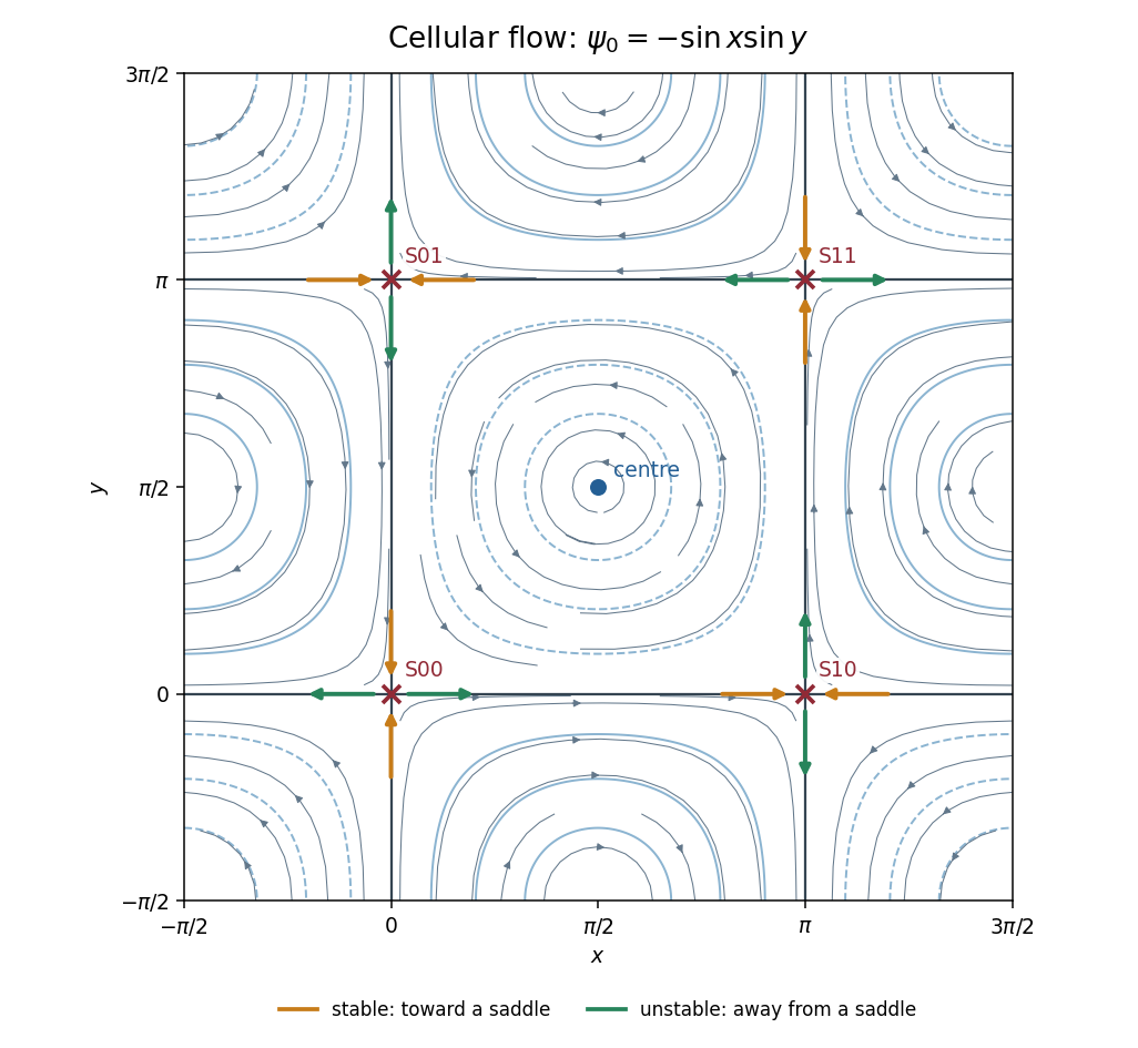
Unperturbed cellular streamlines, four interior saddles, and stable and unstable branches
. Details. 
Use a Poincaré map sampled once per forcing period. A hyperbolic periodic trajectory has stable manifolds containing parcels that approach it under forward iteration and unstable manifolds containing parcels that approach it under backward iteration. In the integrable limit the relevant branches coincide along a heteroclinic orbit and form a barrier between neighboring cells.
A transverse crossing in the perturbed map means that this barrier has split: a parcel on the intersection belongs to both asymptotic manifolds, and adjoining branches enclose fluid lobes transported across the former boundary. Iteration stretches and folds those lobes. In the connected heteroclinic network this creates complicated intercell transport and chaotic advection. The crossing is between invariant curves at the same forcing phase; it does not mean that different trajectories cross at one time in violation of uniqueness.
The incompressible flow gives an area-preserving map, so lobe exchange preserves parcel area. Without diffusion, an advected passive scalar also keeps its value on each trajectory. Therefore manifold intersections can generate fine filaments and efficient advective exchange but do not by themselves produce molecular homogenization, nor prove that every region of the flow becomes chaotic.
Put and . Expansion of the trajectory equation to first order gives, for either correction,Since the unperturbed Hamiltonian flow obeys , differentiation with respect to position yields . Along the heteroclinic orbit this says . Therefore the homogeneous terms cancel:The unperturbed orbit approaches its hyperbolic fixed points exponentially, so at either appropriate endpoint. The selected stable and unstable corrections remain bounded there, approaching the first-order corrections to the periodic trajectories. Their endpoint dot products consequently vanish. Integrating the stable correction forward and the unstable correction backward givesSubtracting proves the heteroclinic Melnikov function for a periodic planar flow:Choose a regular point on the connection where . The first-order signed normal distance between the perturbed invariant curves is . If has a simple zero in the along-orbit parameter, the implicit function theorem continues it to a zero of the actual distance for sufficiently small , with nonzero derivative. The curves consequently cross transversely rather than touching tangentially.
A phase shift and a shift of the reference point along the autonomous connection are equivalent in this calculation: using changes the integrand from to . Thus a simple phase zero can also describe a crossing along the connection at a fixed forcing phase. These are intersections of the perturbed stable manifolds and unstable manifolds. The word “unperturbed” in the printed conclusion cannot be literal: those branches coincide before perturbation and have no transverse splitting.
On , the unperturbed trajectory satisfies . Put . Integration with givesIt runs from to , so it is the appropriate heteroclinic orbit. From the perturbed stream function,On the chosen connection, ; hence the scalar product in the heteroclinic Melnikov function for a periodic planar flow is . ThereforeSet . The odd term integrates to zero, leaving the supplied even Fourier integral multiplied by . ThusFor every fixed the amplitude is nonzero and the phase zeros are simple: there is . At fixed phase, varying also gives simple zeros because is nonzero for . The Melnikov splitting of a periodically perturbed cellular flow therefore produces transverse manifold intersections at sufficiently small perturbation and fluid-lobe exchange between adjacent cells. The unperturbed separatrix is no longer a material transport barrier.
At high frequency the leading splitting amplitude is asymptotic to , so fast forcing has an exponentially weak first-order effect on this connection. This is a fixed-frequency, small- result; an exponentially small leading term need not dominate higher orders in a simultaneous high-frequency limit. At exactly the perturbation itself vanishes and , so the nonzero-frequency conclusion does not apply. Manifold splitting demonstrates intercell chaotic advection locally, not a proof of uniform mixing or ordinary diffusion throughout the entire domain.
Articles by others on the same topic
There are currently no matching articles.