The cellular approximation theorem says that a continuous map between CW complexes is homotopic to a cellular map, meaning that it sends each -skeleton into the target's -skeleton. Give , for , its CW complex structure with one zero-cell and one -cell. Its -skeleton is the whole sphere, so the theorem applies and gives the requested result. For use the two zero-cells of . In particular the conclusion isThere is no local-finiteness assumption on .
For completeness, here is a direct proof of the needed case of cellular approximation, including the point-avoidance step. We use three standard facts, stated explicitly. First, a compact subset of a CW complex lies in a finite subcomplex. Second, a continuous map from a smooth manifold into Euclidean space has arbitrarily close smooth approximations, and smooth cutoffs exist around compact subsets of open sets. Third, the Sard theorem says the critical values of a smooth map have measure zero; when the domain dimension is smaller than the target dimension, its entire image has measure zero.
The first fact has a useful short proof. If a compact set met infinitely many open cells, choose one point in each of countably many distinct cells. Closure-finiteness makes every closed cell meet the chosen set, and every subset of it, in finitely many points. The weak topology of a CW complex then makes all those subsets closed. The chosen set is an infinite closed discrete subset of a compact space, a contradiction. Taking the closures of the finitely many cells met proves the claim.
Now lies in a finite subcomplex . Take a top-dimensional open cell of with , and identify its interior with the open unit ball in using its characteristic map. On the open set , write for the coordinate expression. Choose and a smooth cutoff supported in and equal to one near the compact set . By smooth approximation of maps into Euclidean space, choose a smooth with , where . Replace byThe straight-line interpolation is a homotopy supported away from the boundary of the cell and stays inside that cell. Where , we have and hence . By the Sard theorem, choose outside . Where we have , and elsewhere , so the modified map avoids everywhere.
Radial retraction of onto its boundary fixes that boundary. It therefore descends through the characteristic map, including its possibly noninjective boundary identifications, and fixes all other cells of . Composing gives a homotopy whose endpoint misses all of . Remove every cell of dimension greater than in descending order. There are finitely many such cells, so their homotopies concatenate to yield . This proves dimension reduction of sphere maps into CW skeleta. The approximation step is essential: an arbitrary continuous image of can fill a higher-dimensional region, so dimension alone would not supply an omitted point.
The Morse lemma states that if is a nondegenerate critical point of a smooth real function on an -dimensional smooth manifold, there are smooth coordinates , centered at , such thatHere is the Morse index, the number of negative directions of the Hessian matrix at . The equality is exact on a neighborhood, not merely a second-order expansion.
To prove it, start with any coordinates putting . Since , integral Taylor theorem givesThe matrix is smooth and symmetric, with . By Sylvester's law of inertia, a constant invertible linear coordinate change makes .
We perform completion of squares with coefficients depending smoothly on the original . The first pivot stays nonzero and keeps its sign on a sufficiently small neighborhood. Algebraically,The remaining coefficient matrix is the Schur complement. At zero it is the remaining signed diagonal matrix, so its first pivot is also nonzero nearby. Continue recursively, shrinking the neighborhood finitely many times. Every pivot is smooth and nonzero, with sign for and thereafter. Absorb into the square by its smooth positive square root. This produces a smooth triangular matrix with nonzero diagonal such thatAll coefficients here are functions of the original ; no circular coordinate substitution is involved. Define . Its derivative at zero is , which is invertible. The inverse function theorem makes a smooth coordinate system and gives the asserted exact quadratic form. The number of negative squares agrees with the Hessian matrix signature and hence with the Morse index. This is the smooth completing-square proof of the Morse lemma.
A Morse function is a smooth real-valued function all of whose critical points have nonsingular Hessian matrices. We use the descending convention for a gradient-like vector field : away from critical points, , and near a critical point of Morse index , in Morse lemma coordinates , the field can be chosen as .
For its flow , define the unstable manifold and the stable manifold . Their dimensions are and . The Morse-Smale transversality condition isFor a closed manifold, this lets us form the Morse-Smale complex over . Orient each unstable manifold and takeThe transverse intersection for an index difference of one is one-dimensional; quotienting by flow time gives a finite set of trajectories, and counts them with orientation signs. Compactifying the one-dimensional spaces of trajectories for an index difference of two adds broken trajectories. Their oriented boundary count is zero, giving . The descending cells are the unstable manifolds, and these counts are the incidence numbers of the corresponding cellular chain complex, so the homology of this complex is . Ambient orientability is unnecessary: orientations of the unstable cells provide the requisite coorientations and trajectory signs.
For the Klein bottle, use the quotient of by and . A model of the standard four-critical-point height function isIt is well defined under both identifications. Its critical points, their Morse indices, and critical values areThe Hessian matrix is diagonal with entries and , so each point is nondegenerate. The flat quotient metric gives descending equations , . Their saddle separatrices are the coordinate lines; the two saddle-to-saddle intersections are empty, and all remaining stable and unstable intersections are transverse. This is a Morse-Smale gradient flow. If one insists on the exact local-model version of a gradient-like vector field above, change the two coordinate speeds near the critical points to the standard quadratic-model speeds. This preserves the separatrices, signs and transversality.
Both branches of either saddle flow to the minimum with opposite endpoint signs, so . From the maximum to , the two trajectories lie on and approach from opposite directions. The identification in is a translation, so their incidence signs are opposite and cancel. The two trajectories to lie on and approach from opposite directions. The identification in reverses the transverse -coordinate, reversing one additional orientation sign. These two contributions consequently have the same sign. Choosing the orientation of gives .
One can check the coefficient directly from the cell attachment of the top cell: its boundary word is , with exponent sums zero on the base loop and two on the fiber loop . Thus the integral Morse complex of the Klein bottle isandCounting trajectories without signs, or working only modulo two, would miss the order-two class.
Work over . A closed connected orientable surface of genus has Betti numbers ; the circle has Betti numbers . The Künneth theorem therefore givesWe use the following precise consequence of the Morse handle-attachment theorem: a closed manifold with a Morse function has the homotopy type of a finite CW complex with one index- cell for each index- critical point. Its degree- rational cellular chain group has dimension , so its homology has dimension at most . Consequently , the weak Morse inequalities. Summing yieldsThis counts every critical point, regardless of whether some critical values coincide.
To attain the bound, construct a surface Morse function from the standard orientable handle decomposition: start with a disk, attach orientable bands in the usual paired pattern forming the genus- surface with one boundary component, and cap that boundary with a disk. Give the first disk a minimum, each band one saddle with local form , and the final cap a maximum. Regular collar coordinates join successive levels without additional critical points. This constructs with counts .
On the product takeIts critical points are exactly the pairs of a critical point of with . The Hessian matrix is block diagonal, with surface block and circle entry . It is nonsingular and its Morse index is the sum of the two factor indices. Thus this product of Morse functions has countsand exactly critical points. If distinct critical values are desired, choose outside the finite set producing collisions after first choosing distinct critical values for . The minimal Morse critical count on a circle times an orientable surface is therefore attained for every .
Here projection means Hermitian orthogonal projection: with , as indicated by the unitary conjugation in the question. These matrices represent the complex Grassmannian as orthogonal projections, a compact manifold of complex dimension . The constants are real. Let and use the given tangent directions . Cyclicity of the matrix trace givesThe commutator is skew-Hermitian. If this derivative vanishes for every skew-Hermitian , choose to obtainso . Conversely makes every tangent derivative zero. Because the diagonal entries of are distinct, a commuting matrix is diagonal. Its idempotent entries are zero or one. Thus the critical projections are exactlywith critical points and values .
To compute the Hessian matrix, write and . A neighboring plane is the graph of a complex linear map . With , its orthogonal projection is . Writing for the diagonal blocks, we getExpanding yieldsEach complex coordinate has two real components, each with Hessian coefficient . Every coefficient is nonzero, proving that is a Morse function. Its negative directions correspond to . For there are complementary indices below , givingThis is the diagonal trace Morse function on a complex Grassmannian. Its critical values need not be distinct; ties between sums do not make its critical points degenerate.
All Morse indices are even. Choose a Morse-Smale gradient flow and form its integral Morse chain complex. The odd-degree chain groups vanish, so every differential vanishes. Equivalently the Morse handle-attachment theorem supplies only even-dimensional cells. The integral homology of complex Grassmannians is thereforewhere counts the subsets with , and . In particular there is no torsion. The nondecreasing sequence lies between zero and , so reversing it identifies these subsets with partitions of an integer fitting in a by rectangle. The Poincaré polynomial is explicitlyFor the permitted example , the subsets have indices . ThusThe general calculation above applies throughout ; it does not reduce to any of the excluded rank-one cases.
An index- handle in dimension is . A handle attachment glues its attaching region to a corresponding neighborhood in the boundary of the preceding manifold with boundary. Besides the embedding of the attaching sphere, one specifies a framing of an embedded sphere, namely the normal-disk directions used in this gluing. Corners are then smoothed.
In dimension four, a two-handle is and attaches along . Its attaching circle is a knot in the boundary of the zero-handle . Identify that boundary with and remove a point away from the circles to draw them in . Disjoint attaching circles give a framed link. Each integer records the twist of its normal framing relative to the zero Seifert framing; the integer is also the linking number of the circle and its framed push-off. The resulting boundary change is Dehn surgery on a framed link. This is the two-handle part of a Kirby diagram.
For , use the following explicit handle decomposition. Write each factor as two disks, , glued along their boundary circles. The four product pieces giveThe first is a four-dimensional zero-handle after rounding its corners. Its boundary is the union of the solid tori and . The two middle product pieces attach along these tori. Their attaching circles and form the standard Hopf link, with linking number one after choosing orientations.
Both framings are zero. For example, the normal disk of is the second disk factor. Its constant normal push-off has linking number zero with the original circle: the circle bounds in the four-ball, and a parallel push-off bounds a disjoint translated disk. Thus the framed self-intersection is zero; the same argument applies with the factors interchanged. These product framings are the zero Seifert framings.
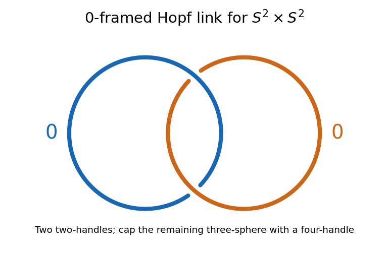
Zero-framed Hopf link for the two two-handles of S2 times S2; the upper crossing has blue over orange and the lower crossing has orange over blue
. Details. 
After these two two-handles, the remaining product piece is a four-ball. Its boundary is exactly the boundary of the assembled first three pieces, so it attaches as a four-handle. Equivalently, zero surgery on the Hopf link gives , which this handle caps. We have therefore constructed the actual product, provingThere are no one- or three-handles. As a check, the two factor spheres have self-intersection zero and meet once, giving the intersection form . The explicit product construction, rather than the intersection form alone, identifies the smooth four-manifold. This is the zero-framed Hopf-link handle decomposition of the sphere product.
Articles by others on the same topic
There are currently no matching articles.