At both points, and , so both components of the vector field vanish. Thus both points are equilibrium points for every parameter value. These are regular points of the spherical coordinates chart: the coordinate singularity at the pole plays no role in their linearization.
Use local coordinates , at . The Jacobian matrix, its trace and its determinant areConsequently is attracting when , repelling when , and a saddle equilibrium when . A transition between a node and a focus at changes the linear geometry but is not a bifurcation of the local topological phase portrait.
The stationary bifurcation curve is . To identify it, write , . At a non-equatorial equilibrium point, eliminating givesNear , if , these yield and . The two branches are related by the local reflection . Their determinants are , so they are saddle equilibria. This is a pitchfork bifurcation; on the portion with the saddle branches lie on the side where is stable, giving a subcritical pitchfork bifurcation.
A Hopf bifurcation requires , henceThe oscillation frequency is . At the intersection , but : there is a double zero eigenvalue with one eigenvector. The map from to has nonzero Jacobian determinant, so two independent parameter conditions produce this codimension-two bifurcation. Reflection removes quadratic terms; the appropriate initial comparison is with a reflection-symmetric cubic double-zero normal form, subject to the cubic degeneracy checked below.
For completeness, the printed vector field has a subcritical, rather than supercritical, Hopf bifurcation. In the mechanical coordinates , , at its cubic acceleration has coefficient and coefficient . For a small harmonic oscillation, the averaged cubic change of is , whereThus a small unstable periodic orbit lies on the attracting side of the Hopf bifurcation. This calculation matters when comparing the original equations with the later assumed normal form.
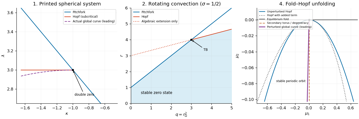

The cubic Taylor expansion at the double-zero point isThere are no quadratic or quartic terms because the local vector field is odd under . Set , , and use . The linear transformation is invertible, and the positive time rescaling preserves orbit orientation. With primes denoting , the result isThis supplies the requested cubic functions, with a remainder stronger than .
There is an important normal form check. Setting , straightens the first equation, and differentiating givesIn particular the nilpotent cubic damping invariant is . A nonsingular cubic near-identity transformation and rescaling cannot change this vanishing invariant into the nonzero coefficient in the supplied later normal form. The conclusions for that assumed system are therefore given separately from the independently derived conclusions for the printed original equations.
First analyze the supplied normal form as a dynamical system in its own right. Its equilibrium points are and, for , . At , the trace is and the determinant is . At , the determinant is , so both are saddle equilibria. Thus is the pitchfork bifurcation curve, and is the Hopf bifurcation curve. With the allowed supercritical Hopf bifurcation, an attracting limit cycle is born on around the repelling origin.
The Hamiltonian obeys . Set , , , , and . The limiting Hamiltonian system has two oppositely directed heteroclinic orbits with for . The Melnikov energy-balance method givesIts unique simple zero gives a heteroclinic cycle curveThe two connections occur on the same curve because reflection interchanges them. The attracting limit cycle grows toward this heteroclinic cycle, then disappears. In the small unfolding neighborhood there is one such connection curve, rather than two independently split curves. There are no nearby homoclinic orbits replacing it: the two equal-height outer saddles are the relevant separatrix endpoints.
This calculation transfers to the original equations only if the asserted reduction is valid. The cubic calculation in part (c) shows it is not valid for the printed coefficients. Nevertheless, the claim of a single nearby global bifurcation curve for the original equations can be proved independently. Put , , , , and . Eliminating using producesThe order- correction is reversible and has no first-order separatrix energy imbalance. On the limiting positive connection, and . The first dissipative balance isAgain the zero is simple, and reflection makes the two heteroclinic orbits simultaneous. Hence the actual original equations have the unique local connection curveThe unstable limit cycle on the subcritical Hopf bifurcation side reaches this curve. Thus the original system still has one nearby global connection curve, but its tangency and cycle stability differ from those of the supplied assumed cubic normal form. These statements concern connections contained in the shrinking neighborhood of ; they do not exclude unrelated distant global bifurcations elsewhere on the sphere.
For the supplied normal form, the four local topological phase portraits are as follows. When , only the origin is present and it is a saddle equilibrium. When , the origin is attracting, between the two outer saddle equilibria; inward-facing separatrices enter its basin. When and , the origin is repelling and a stable limit cycle surrounds it, inside the separatrix boundary formed by the outer saddle equilibria. Finally, when , the origin remains repelling but the local limit cycle has disappeared, and trajectories leave the central region through the opened separatrix channels. Whether the origin is a node or a focus within one of these regions does not change this orbit topology.
On the connection curve, the two outer saddle equilibria are joined in both directions; the period of the disappearing limit cycle diverges. This is a heteroclinic cycle, not a pair of saddle homoclinic orbits. The sketches below show the four open regions of the supplied system; they are not presented as phase portraits of the inequivalent printed spherical equations.
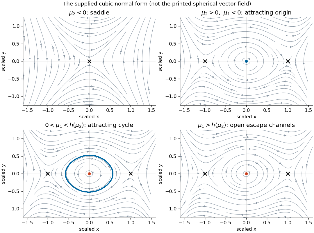
Four phase portraits of the supplied reflection-symmetric cubic normal form
. Details. 
Articles by others on the same topic
There are currently no matching articles.