Take at the base and assume gas leaves freely at the liquid surface, without being retained as foam. There is no new bubble production after filling. Neglecting the liquid velocity, gas-volume conservation is a scalar conservation lawAn impermeable base has no incoming bubbles. Thus a clear region develops below the uniform bubbly region. The clearing discontinuity satisfies the Rankine-Hugoniot condition, with states and :For the dilute regime , the characteristic speeds obey , so this is the admissible compressive shock. Before it reaches the surface,The remaining bubbles move upwards at and escape at the top. Averaging the void fraction over the entire cylindrical volume givesThis bubble clearing in a cylindrical vessel describes bubbles in the liquid, not a hypothetical retained gas layer above it. A closed surface or long-lived foam would require a different upper boundary condition.
The radius law integrates to , so the cross-sectional area is . Conserving gas volume in a horizontal slice yieldsor the kinematic bubble transport in an exponentially narrowing vessel equationThe geometrical term increases the concentration as a given gas flux enters a smaller area. On concentration characteristic curves,Put . A characteristic starting at with hasThe first formula follows by integrating ; inserting it into gives the second. For initially uniform , the uninterrupted bubbly region remains spatially uniform, with this time-dependent concentration. These characteristic curves carry concentration information; they are not individual bubble trajectories, whose speed is .
Use the uniformly filled narrowing vessel of the preceding part. A bubble within its uniform bubbly region seesIts material rise speed is , not the concentration-characteristic speed. Integrating from givesThe cylindrical limit is , as required. The bottom clearing front follows this same position by the local Rankine-Hugoniot condition. In the narrowing vessel the formula applies until the bubble leaves at , or a boundary interaction changes the uniform state. Its formal large-time limit is , while . Crowding and liquid backflow invalidate the assumed dilute, negligible-liquid-velocity closure before this limit is a reliable prediction of a real tankard.
The Rayleigh number compares destabilizing thermal buoyancy with viscous and thermal diffusion:The conductive heat flux is , and the Nusselt number is the actual upward heat flux divided by this value. The four-thirds convective heat-transfer law is the empirical large-Rayleigh closure . It givesThe layer depth cancels: thin thermal boundary layers control the resistance while convection mixes the interior. The dimensionless coefficient depends on the boundary and material-property regime; the two boundary-layer temperature drops can be absorbed into its convention. This is not a universal law for all Rayleigh-Bénard convection. Below convective onset the stable conductive solution instead has , and an impulsive initial conductive transient is not described by the steady large-Rayleigh closure.
Cooling from above makes dense cold fluid overlie lighter warm fluid, so the upper boundary layer is unstable and can mix the interior. Assume high Rayleigh number, rapid interior mixing, constant properties, negligible wall heat capacity and a quasi-steady cooling flux obeying the four-thirds convective heat-transfer law. Write and use a coefficient appropriate to this single cooling boundary. The volumetric heat capacity is , so the area-wise heat balance isWith , integration gives convective cooling under the four-thirds heat-transfer law:The power-law decay is a bulk approximation between the initial boundary transient and the later stage when the decreasing temperature contrast no longer maintains strong convection. It is not an exact spatially uniform solution satisfying the cold boundary itself.
Cooling from below is different: dense cold fluid now lies below warm fluid and stabilizes the layer. With no other imposed motion, cooling is by thermal conduction, and temperature becomes depth dependent. Let be the cooled bottom and the insulating top. Solve with , and . The mixed-boundary eigenfunctions have , givingIts volume-averaged temperature isThe late conductive decay is exponential on the timescale , rather than the convective bulk law. This assumes the usual positive thermal expansion coefficient and no destabilizing compositional stratification.
The shallow-water approximation requires the depth to be small compared with the horizontal scale of variation, small vertical accelerations and nearly hydrostatic pressure. Take cross-sectionally uniform lower-layer velocity and a sufficiently deep, effectively stationary upper layer. Under the Boussinesq approximation, is the reduced gravity. Conservation of lower-layer volume gives constant discharge .
Dividing the Bernoulli equation by gives the shallow-water specific energyAt fixed , the energy curve has its minimum at the critical depth , where . Above this minimum there are two depth branches: deeper subcritical flow has , and shallower supercritical flow has .
The two long-wave speeds relative to the bed are . In subcritical flow one family can propagate upstream and one downstream; in supercritical flow both travel downstream for . At hydraulic control, , and a smooth transcritical solution must also satisfy the geometric regularity condition. The flow may remain entirely on either branch, cross smoothly through the control from subcritical to supercritical, or take the reverse smooth branch under appropriate boundary conditions. A downstream hydraulic jump can return supercritical flow to the subcritical branch while losing energy.
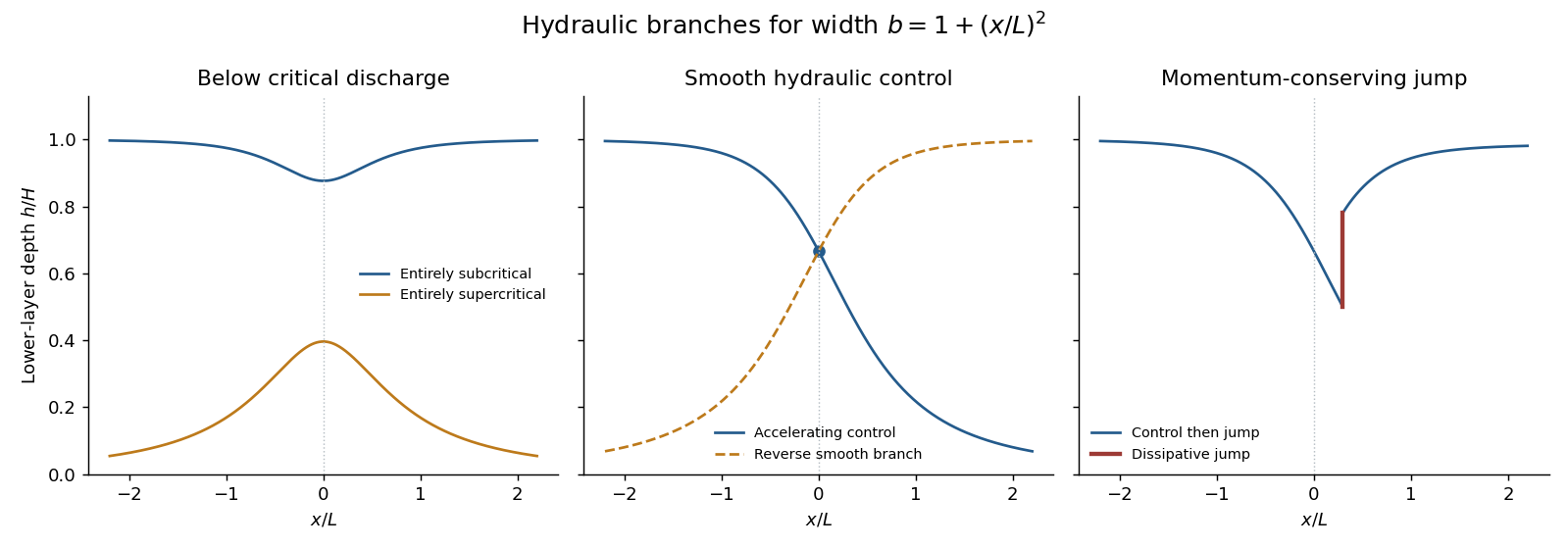
Depth branches in a contracting and expanding channel, including hydraulic control and a dissipative hydraulic jump
. Details. The sketch distinguishes smooth branch changes at a critical section from a jump: a jump conserves mass and momentum, not the original Bernoulli head.
Differentiate the specific energy at fixed discharge:In the lossless flat channel is constant. A smooth hydraulic control has , so regularity requires . For the prescribed width this occurs at the minimum width . The required minimum specific energy is largest at the narrowest section; a controlled flow supplies exactly that head.
Far upstream , so the velocity of a finite-discharge flow with depth tending to tends to zero. Thus the Bernoulli equation gives . At the control and , henceThe printed width normalization has . Downstream on the accelerating controlled branch the flow becomes shallower and supercritical.
Assume the jump is stationary, short compared with the scale of width variation, hydrostatic on either side, and has negligible bed stress integrated over its short length. Treat its width as constant. It must occur on the downstream supercritical branch, at . The discharge from the control gives the local unit-width dischargeBefore the jump the energy is still . Writing , its equation is . Its positive roots are and ; the former is supercritical. ThusMass conservation gives . The hydraulic jump momentum balance conserves . Factoring out the non-jump solution gives the conjugate-depth relationConsequently the conditions immediately after the jump areIts Froude number is below one. The specific-energy loss isSelecting the deeper root of the unchanged energy equation would be wrong: that would conserve the energy across a turbulent jump instead of the momentum.
Bed and sidewall stress, turbulent mixing at the interface, wave radiation and hydraulic jumps convert or remove mechanical energy. In the specified local head-loss model, differentiate while keeping constant:At a regular hydraulic control the coefficient of vanishes. Therefore requiresThus the control moves to the widening downstream side, . This is the exact local compatibility condition; it is the head-loss correction to hydraulic control with loss expressed as Bernoulli potential per unit length.
For a small loss and a control remaining near the throat, use the lossless depth and . The leading displacement isFor a finite loss, the local derivative alone does not specify the accumulated loss from the far-upstream reservoir, so it does not fix a unique revised discharge or numerical control depth. Given , the exact condition can instead be solved implicitly for ; if the inviscid discharge is imposed, it becomes . The small-displacement root is the one continuous from the throat. This distinction avoids treating the original upstream energy as unchanged after an unspecified finite upstream loss.
Use the explicit printed width law . Its wetted area and hydrostatic pressure integral areAssuming hydrostatic pressure, a horizontal prismatic bed and cross-sectionally uniform velocity, volume conservation and momentum conservation give the prismatic-channel shallow water equationsEquivalently,The coefficient matrix in variables is . Its eigenvalues and the corresponding gravity-wave speed areFor these eigenvalues are distinct and real, establishing strict hyperbolicity in the hyperbolic partial differential equation sense. Since , substitution in the two equations showsFor example . This provides both the slopes and the conserved characteristic quantities. At a dry bed , strict hyperbolicity degenerates and the front is interpreted as the limit from positive depth.
The descriptive word “parabolic” alone would normally suggest and different coefficients. The explicit width in the PDF determines the calculation here; it must not be silently replaced by that other geometry.
Put the broken dam at and let . A dry bed is assumed downstream. The left-family rarefaction wave joins the undisturbed reservoir to the dry front. The other Riemann invariant is fixed at . Within the fan its characteristic speed equals , soThus the dry-bed dam break with cubic wetted area has the fieldsVelocity is not a meaningful fluid quantity in the dry region; its wet-side limiting value is . The upstream head travels at , while the front travels at the stated constant speed in this inviscid model.
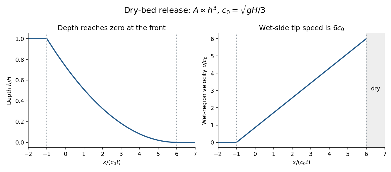
Bottom drag slows the flow and changes the dry-tip structure, where the depth is small and bed stress per unit fluid mass becomes especially important. It can replace the inviscid zero-depth high-speed tail by a drag-controlled nose. An exact altered profile or front speed requires a specified drag law; the inviscid speed should not be extrapolated to a thin real irrigation-channel front without that qualification.
Treat the newly placed sand barrier as impermeable during the initial release. The downstream isolated reservoir occupies with depth and has finite volume . The remaining upstream water stays behind the barrier; it does not continuously feed the released region. Assume so that the shallow-water approximation is appropriate.
Until the rarefaction head reaches the barrier atthe previous dam-break solution is unchanged on the released side. The wall imposes . After , a reflected downstream family adjusts the flow near the wall. It is a lowering/depletion adjustment, not a new upstream supply. The upstream depth decreases, the finite water volume spreads downstream, and the unmodified simple-wave region shrinks relatively.
The leading characteristic of this adjustment can be determined exactly without solving the whole reflected region. In the still-unmodified fan,Integrating gives the finite-reservoir reflection of a cubic-area dam-break rarefaction:The solution to the right of this curve is still the original fan. Crucially at every finite time. Therefore the ideal inviscid dry tip remains at : finite reservoir volume does not by itself justify an immediate change to that front law. Only a vanishingly small amount of fluid occupies its very thin forward tail at late times. Bottom drag, leakage or other front physics changes this conclusion.
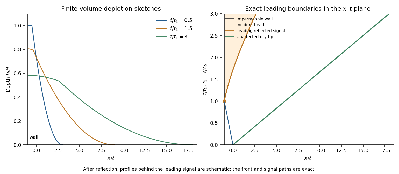


The profiles behind the reflected edge are schematic; there the two characteristic families interact and the original one-invariant fan no longer supplies the complete fields. The x–t diagram distinguishes the wall, the incident head, the exact reflected leading edge and the unaffected dry-tip trajectory.
Assume quasi-steady saturated Darcy flow, hydrostatic pore pressure, a long shallow barrier, isotropic intrinsic permeability of a porous medium , an impermeable lined base, and negligible capillarity. Maintain upstream and downstream free-surface heads at and . The Dupuit approximation neglects vertical velocity except in small entrance/exit regions. Let be the fluid's dynamic viscosity and its hydraulic conductivity.
Since the pressure is , the superficial Darcy velocity is , uniform with depth at fixed . Integrating over the printed channel width givesThe steady discharge is constant, so integration with the two head boundary values gives Dupuit flow in a channel with cubic wetted area:Here is total volume per time, including the changing channel width. The pore-space mean speed is . Thus porosity affects storage and pore transit time but does not separately multiply this steady discharge when is the intrinsic permeability in Darcy's law. If “permeability” is instead supplied as hydraulic conductivity, use that value directly for . An exact seepage-face/free-boundary calculation near the outlet would go beyond the shallow Dupuit model.
Because , the lower layer is saturated along the entire barrier. Both layers have the same horizontal head gradient but different Darcy velocities. Integrating their conductivity over the actual cross-section gives the transmissivityThe total discharge is . Hence , givingThis is a parallel-layer conductivity integral, not a series-resistance average: the layers share the horizontal pressure drop. It reduces to the previous result when . The assumption is important; if the downstream free surface cuts the lower layer, the transmissivity and its head integration must be split into different saturation regimes.
Use the flux normalization of the supplied equations, with the common factor suppressed. Put , and . The top-hat plume model reduces toEliminate height to obtain . Integrating with zero source volume and momentum flux gives the pure plume balanceEquivalently, seek and . The volume balance gives , and the momentum and buoyancy balances give and . ThusA finite source replaces the singular point origin by a plume virtual origin and source conditions. The Boussinesq approximation requires the fractional density difference to be small, so density can be replaced by ambient density in inertia and entrainment while retaining the small difference in buoyancy. In this solution it requires . The approximation necessarily fails sufficiently near the ideal point source, where diverges, and can also fail for strongly heated or otherwise large-density-contrast sources. The similarity solution is appropriate farther away once entrainment has diluted the anomaly, assuming a uniform ambient, constant entrainment coefficient and negligible confinement, heat loss and stratification.
The mass and heat entrainment equations immediately giveUse the specified relation . ThenMeanwhile the kinematic buoyancy flux isSince , and are constant,Thus conservation is a consequence of conserved excess heat in this ideal-gas, uniform-ambient model, not merely an assumption that arbitrary non-Boussinesq buoyancy fluxes are conserved in every environment.
From the definitions of mass and momentum fluxes,The density relation follows by solving the conserved-buoyancy identity in the preceding part. Hence andThe second equality uses and .
Set and . The equations become , , exactly the same flux system as for the pi-suppressed Boussinesq pure plume. For the heated point source take zero initial mass and momentum flux and the finite conserved heat/buoyancy supply. DefineThe resulting mass and momentum fluxes areSubstituting into the density relation gives the non-Boussinesq pure-plume density transitionThe two expressions for agree because . Density increases from the very dilute near-source regime toward the ambient value as entrainment increases the mass flux.
The flux solution gives , while . ThusAt , , and . This height marks the transition between a strongly non-Boussinesq near-source plume and the dilute far-field plume. For , and , recovering the Boussinesq solution. For , , and .
The ideal point-source limit still has a divergent velocity and temperature; it is not a literal resolved finite burner. In particular, zero source mass flux does not imply zero physical hot-gas volume flux: tends to in this limiting solution. Source size, compressibility and heat transfer impose additional near-source limits on the model.
Assume Boussinesq approximation, no wind, a uniform exterior, negligible source volume, sharp well-mixed internal layers, point-source pure plume entrainment and thin openings represented by discharge coefficients . Let be the upper-layer reduced gravity. Steady volume conservation makes the magnitudes of inlet and outlet flow equal to .
If the opening pressure drops are and , the orifice laws and hydrostatic pressure difference giveDefine the reduced area byThen the throughflow in this displacement ventilation model isLower-layer conservation requires . Global buoyancy conservation gives . Eliminating yieldsThis uniquely determines an interface height between zero and for a given positive area parameter. Opening area controls the nondimensional height; source strength controls the density contrast and flow magnitude. Factors of two depend on the stated effective-area convention, which has been fixed explicitly here.
Let denote the density deficit of each warm layer relative to outside. The integrated hydrostatic driving head isThe same pair of orifice laws therefore givesBoth plumes remove fluid from the lower layer. If and are their fluxes at its upper interface, lower-layer conservation also givesIn steady state the weak plume supplies the middle layer, while the strong plume entrains that supply above and carries the total volume into the upper layer. Consequently and . These balances assume the plumes remain spatially separate and wall heat loss is negligible.
Put . The middle layer matches the density of plume 1 at , so . The upper layer exports both sources, so . With and , the two-plume three-layer displacement ventilation density ratio isThe driving head can therefore be rewritten as , whereCombining with gives . But , and henceThe square root requires a positive remaining buoyancy head.
As , the weak source vanishes and : the middle and lower layers have the same density, leaving a single physical interface at . The old no longer marks an independent density interface. The single-plume two-layer model is the meaningful limit; the additional closure in part (e) also gives .
As , the density ratio tends to one, so the middle and upper layers merge. There is then a single physical lower interface , fed by two equal, separate plumes. The area prefactor tends to two and the head reduces to . The mathematical label ceases to identify a distinct density interface, so a finite limiting value assigned to it by an extra closure is not evidence for three distinct layers. Two separate equal plumes entrain more than one coincident plume of combined source strength; the distinction survives after the layers merge.
Above , plume 2 entrains middle-layer fluid rather than the original ambient. That fluid is already warm and light, so the plume's buoyancy relative to its surroundings is reduced. Its pre-interface density contrast and zero-source pure plume formula cannot simply be continued unchanged through the interface.
A consistent model treats the middle layer as a uniform new ambient, assumes a sharp interface and weak overall density differences, and carries the incident volume and momentum fluxes continuously across it. The relative buoyancy flux immediately above the interface isContinue an entraining plume model from these nonzero incident fluxes, using buoyancy measured relative to the middle layer. In that uniform layer the relative buoyancy flux is conserved, while entrainment raises the absolute buoyancy carried relative to the outside environment. This is generally a finite-flux or forced plume continuation, not a newly reset point-source similarity solution. A virtual-origin approximation can be used only after matching its fluxes appropriately.
At its matching level , the plume density reaches the upper-layer density; it spreads and detrains, with possible finite-momentum overshoot. The model neglects mutual plume entrainment, wall heat transfer, interface thickness and detailed intrusion dynamics, and assumes each ambient layer is well mixed. In the equal-source limit , the continuation is a neutrally buoyant momentum-driven flow, emphasizing why the upper interface loses its independent density meaning.
The strong plume's outgoing flux equals the total lower-layer supply, . Apply the additional closure in this part and the lower-layer balance from part (b):Dividing by givessoFor this puts the second matching level above the first. It tends to one as and to as . At the latter endpoint the two warm layers already have identical density, so is only a formal matching label, not a distinct observable interface. The expression follows from the stipulated closure; modeling the actual plume in the changed ambient requires the matched continuation discussed in part (d).
Articles by others on the same topic
There are currently no matching articles.