An order parameter distinguishes phases macroscopically. In an Ising model it is the local coarse-grained magnetization; the uniform mean is . In a selected ordered phase , whereas the disordered phase has at zero conjugate field. The ordered signs are related by spin inversion symmetry. A finite zero-field system may average both signs to zero, so spontaneous symmetry breaking is defined using the thermodynamic limit before removing a symmetry-selecting field. For other systems the order parameter can be a vector, a density difference, or a tensor rather than a single magnetization.
Landau-Ginzburg theory makes the order parameter a spatial field and expands a local free energy consistent with the symmetries. For a short-range scalar system with spin inversion symmetry at , a useful expression isThe linear source is the field conjugate to an order parameter. Odd terms at zero field are forbidden by spin inversion symmetry. The coefficients depend smoothly on control parameters away from singular fluctuation effects. With the quartic term suffices locally; if , take for stability. The Landau approximation minimizes this functional; statistical field theory also integrates fluctuations about those minima.
A continuous phase transition has a continuously vanishing order parameter and no latent heat. A first-order phase transition exchanges globally stable phases with discontinuous first derivatives of a thermodynamic potential; the order parameter generally jumps, and an entropy jump gives latent heat. In Landau theory the distinction is determined by global minima, not just by the appearance of additional stationary points.
For the uniform scalar potential with and , its stationary equation is . For , is the minimum; for , the minima are . They approach zero continuously as , giving an ordinary continuous transition.
For and , use the sextic potential. Write . Stationarity of a nonzero phase requires , while equality of its potential with requires . Eliminating yieldsAt this value the potential factors as , proving that the three stationary zeros really are degenerate global minima. Crossing this line makes the order parameter jump: the transition is first order. The disordered and ordered spinodal points instead occur at and respectively, delimiting metastability; these are not the equilibrium transition. If the symmetry allows a cubic term, that term can also produce a first-order transition.
The Maxwell construction replaces a nonconvex homogeneous free-energy density by its coexistence envelope. If excludes the source, the coexisting values satisfyThus one straight line is tangent at both endpoints. Equivalently,the equal-area form of the common-tangent construction. At fixed average between the endpoints, the lever rule gives . Such a mixture has the tangent-line bulk energy, below the energy of an unstable homogeneous state.
The two phases occupy spatial domains separated by domain walls. The gradient term gives a positive wall energy, but a macroscopic interface has area of order rather than bulk volume , so its cost per volume vanishes in the thermodynamic limit. For the symmetric quartic example a scalar quartic domain wall obeys and interpolates between as , with and . Multiplication of the differential equation by gives the first integral , explaining the finite positive interface cost. A uniform unconstrained system need not form both domains: phase separation is particularly relevant when the average order parameter is fixed or boundaries enforce competing phases.
Hysteresis occurs when the system follows a metastable local minimum after another minimum has become the equilibrium one. For , the equation of state is . The hysteresis spinodals of a scalar quartic potential follow from :Following local minima until these limits gives different switching fields on increasing and decreasing . Equilibrium instead switches at . Actual switching can occur before a mean-field spinodal through nucleation, and depends on time scales; hysteresis is not a property of a globally minimized equilibrium potential. The second panel below distinguishes the local branches and their limiting switches.
Critical exponents describe leading singular powers near a continuous phase transition. For reduced temperature , common definitions are the spontaneous order parameter , magnetic susceptibility , singular heat capacity , correlation length , and the critical equation of state . At criticality the connected correlation function has decay power .
In Landau theory, solve the stationary equation, evaluate its stable minimum, and differentiate with respect to the conjugate variables. For a scalar quartic theory with , , the equation of state is . Its ordered solution and differentiated response give and , calculated explicitly in the unheaded solution below. At the same equation gives . The minimized zero-field singular potential is zero above the transition and below, giving a heat-capacity jump and . Expanding the gradient functional about a stable minimum gives inverse quadratic response , so and the Gaussian critical decay has .
These are mean-field critical exponents. Renormalization group methods obtain fluctuation-corrected powers from fixed-point scaling dimensions; they need not equal the Landau values below the upper critical dimension. At a marginal dimension logarithms can supplement the leading powers.
A tricritical point occurs when a first-order boundary meets a continuous-transition boundary. In the spin-inversion-symmetric sextic Landau free energy, two independent parameters must tune , while keeps the potential stable. In the plane, the continuous boundary is , and the first-order boundary is . They meet at the tricritical point; the order-parameter jump on the first-order side tends to zero as . The first panel shows this phase diagram, including the metastability limits derived above.
Along the tuned line , the equation of state is . Thus on a selected ordered branch, rather than the ordinary square-root behavior. Differentiation gives inverse magnetic susceptibility above and below, while at criticality . Hence the mean-field tricritical exponent calculation yields , , ; the minimized potential also gives . These tricritical powers require tuning the quartic coefficient, not merely varying a generic temperature path. The ordinary scalar exponents requested separately are calculated next.
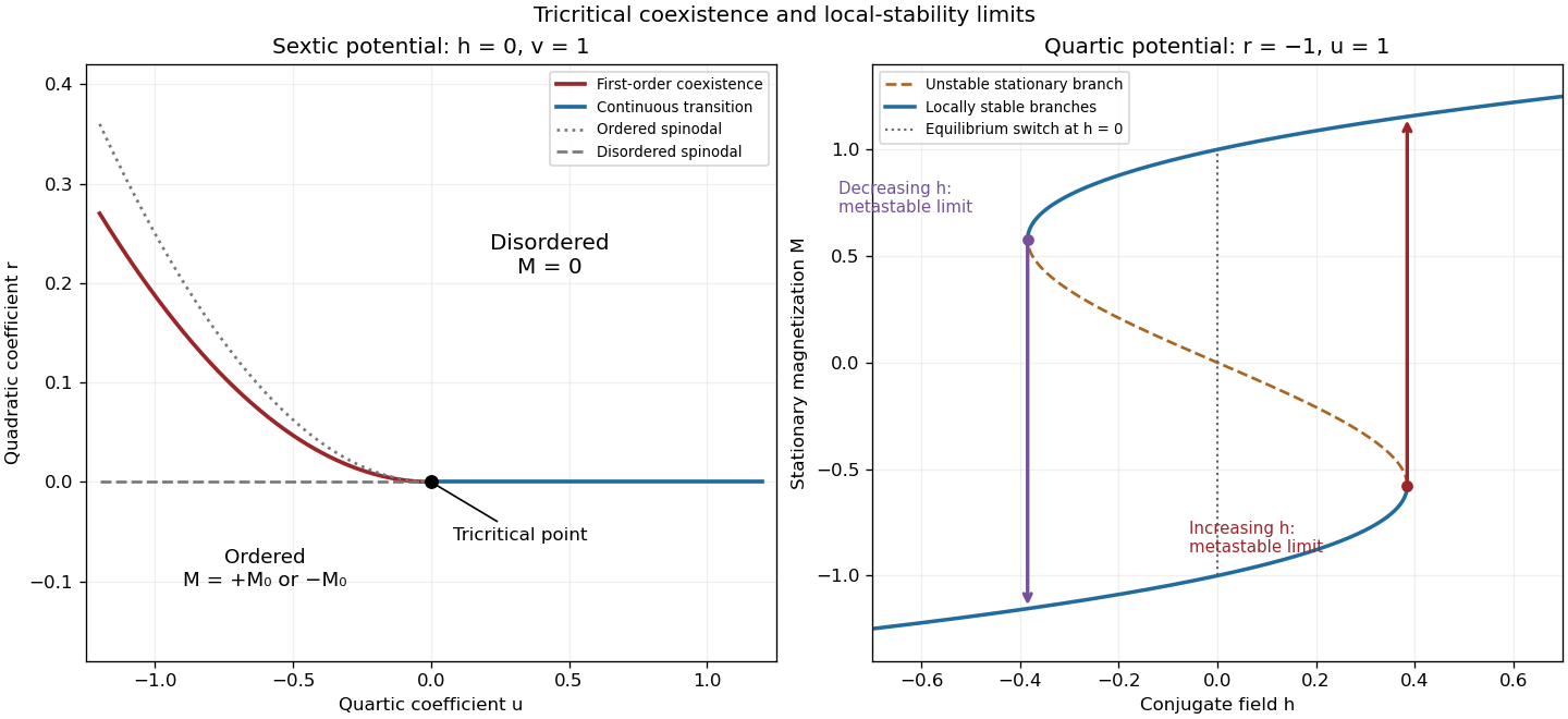
Scalar sextic Landau phase diagram with a tricritical point, and quartic metastable hysteresis branches
. Details. 
For the requested ordinary critical point take , , and the quartic Landau free energy . At , minimization gives . Choosing the positive pure thermodynamic phase,For the magnetic susceptibility, differentiate the equation of state at fixed temperature:Both sides diverge as , with different amplitudes, soThe one-sided field limit below the transition selects a pure phase; differentiating the symmetric finite-volume mixture would instead include its macroscopic switching response.
Articles by others on the same topic
There are currently no matching articles.