An order parameter distinguishes phases macroscopically. In an Ising model it is the local coarse-grained magnetization; the uniform mean is . In a selected ordered phase , whereas the disordered phase has at zero conjugate field. The ordered signs are related by spin inversion symmetry. A finite zero-field system may average both signs to zero, so spontaneous symmetry breaking is defined using the thermodynamic limit before removing a symmetry-selecting field. For other systems the order parameter can be a vector, a density difference, or a tensor rather than a single magnetization.
Landau-Ginzburg theory makes the order parameter a spatial field and expands a local free energy consistent with the symmetries. For a short-range scalar system with spin inversion symmetry at , a useful expression isThe linear source is the field conjugate to an order parameter. Odd terms at zero field are forbidden by spin inversion symmetry. The coefficients depend smoothly on control parameters away from singular fluctuation effects. With the quartic term suffices locally; if , take for stability. The Landau approximation minimizes this functional; statistical field theory also integrates fluctuations about those minima.
A continuous phase transition has a continuously vanishing order parameter and no latent heat. A first-order phase transition exchanges globally stable phases with discontinuous first derivatives of a thermodynamic potential; the order parameter generally jumps, and an entropy jump gives latent heat. In Landau theory the distinction is determined by global minima, not just by the appearance of additional stationary points.
For the uniform scalar potential with and , its stationary equation is . For , is the minimum; for , the minima are . They approach zero continuously as , giving an ordinary continuous transition.
For and , use the sextic potential. Write . Stationarity of a nonzero phase requires , while equality of its potential with requires . Eliminating yieldsAt this value the potential factors as , proving that the three stationary zeros really are degenerate global minima. Crossing this line makes the order parameter jump: the transition is first order. The disordered and ordered spinodal points instead occur at and respectively, delimiting metastability; these are not the equilibrium transition. If the symmetry allows a cubic term, that term can also produce a first-order transition.
The Maxwell construction replaces a nonconvex homogeneous free-energy density by its coexistence envelope. If excludes the source, the coexisting values satisfyThus one straight line is tangent at both endpoints. Equivalently,the equal-area form of the common-tangent construction. At fixed average between the endpoints, the lever rule gives . Such a mixture has the tangent-line bulk energy, below the energy of an unstable homogeneous state.
The two phases occupy spatial domains separated by domain walls. The gradient term gives a positive wall energy, but a macroscopic interface has area of order rather than bulk volume , so its cost per volume vanishes in the thermodynamic limit. For the symmetric quartic example a scalar quartic domain wall obeys and interpolates between as , with and . Multiplication of the differential equation by gives the first integral , explaining the finite positive interface cost. A uniform unconstrained system need not form both domains: phase separation is particularly relevant when the average order parameter is fixed or boundaries enforce competing phases.
Hysteresis occurs when the system follows a metastable local minimum after another minimum has become the equilibrium one. For , the equation of state is . The hysteresis spinodals of a scalar quartic potential follow from :Following local minima until these limits gives different switching fields on increasing and decreasing . Equilibrium instead switches at . Actual switching can occur before a mean-field spinodal through nucleation, and depends on time scales; hysteresis is not a property of a globally minimized equilibrium potential. The second panel below distinguishes the local branches and their limiting switches.
Critical exponents describe leading singular powers near a continuous phase transition. For reduced temperature , common definitions are the spontaneous order parameter , magnetic susceptibility , singular heat capacity , correlation length , and the critical equation of state . At criticality the connected correlation function has decay power .
In Landau theory, solve the stationary equation, evaluate its stable minimum, and differentiate with respect to the conjugate variables. For a scalar quartic theory with , , the equation of state is . Its ordered solution and differentiated response give and , calculated explicitly in the unheaded solution below. At the same equation gives . The minimized zero-field singular potential is zero above the transition and below, giving a heat-capacity jump and . Expanding the gradient functional about a stable minimum gives inverse quadratic response , so and the Gaussian critical decay has .
These are mean-field critical exponents. Renormalization group methods obtain fluctuation-corrected powers from fixed-point scaling dimensions; they need not equal the Landau values below the upper critical dimension. At a marginal dimension logarithms can supplement the leading powers.
A tricritical point occurs when a first-order boundary meets a continuous-transition boundary. In the spin-inversion-symmetric sextic Landau free energy, two independent parameters must tune , while keeps the potential stable. In the plane, the continuous boundary is , and the first-order boundary is . They meet at the tricritical point; the order-parameter jump on the first-order side tends to zero as . The first panel shows this phase diagram, including the metastability limits derived above.
Along the tuned line , the equation of state is . Thus on a selected ordered branch, rather than the ordinary square-root behavior. Differentiation gives inverse magnetic susceptibility above and below, while at criticality . Hence the mean-field tricritical exponent calculation yields , , ; the minimized potential also gives . These tricritical powers require tuning the quartic coefficient, not merely varying a generic temperature path. The ordinary scalar exponents requested separately are calculated next.
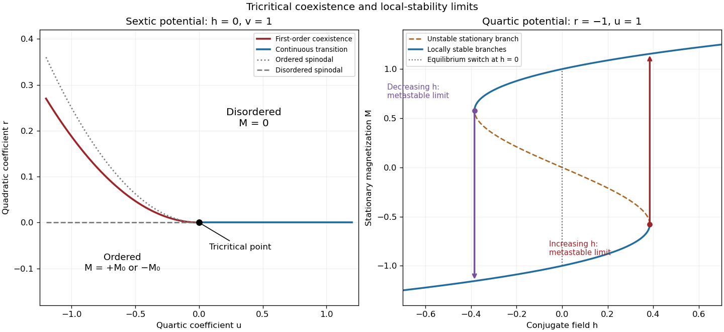
Scalar sextic Landau phase diagram with a tricritical point, and quartic metastable hysteresis branches
. Details. 
For the requested ordinary critical point take , , and the quartic Landau free energy . At , minimization gives . Choosing the positive pure thermodynamic phase,For the magnetic susceptibility, differentiate the equation of state at fixed temperature:Both sides diverge as , with different amplitudes, soThe one-sided field limit below the transition selects a pure phase; differentiating the symmetric finite-volume mixture would instead include its macroscopic switching response.
Use for inverse temperature to distinguish it from the order-parameter exponent. The decaying two-point correlation function needed for the response identity is connected:Away from the critical point in a short-range Ising model pure phase, the correlation length controls the exponential long-distance falloff, with a possible algebraic prefactor. The full two-spin expectation below the transition instead tends to . The spin-mixture contribution to zero-field susceptibility explains why a symmetric mixture is unsuitable for defining a finite connected correlation length in the ordered phase.
Let be the total Helmholtz free energy. Take magnetization and susceptibility per site, soDifferentiating the Boltzmann weights at fixed temperature givesTranslation invariance then yields the correlation-function susceptibility sum ruleTotal magnetization and total susceptibility multiply these expressions by ; per physical volume they have an additional factor relative to the per-site convention. These normalizations do not change the critical powers.
For the subsequent scaling requests, let denote singular free energy per site; the fixed extensive normalization is suppressed. The labels and denote and , with distinct scaling functions and amplitudes on the two sides. Below the transition a one-sided derivative at selects a spontaneous-magnetization branch. Writing , differentiation of the scaling hypothesis for critical phenomena givesThe field-independent makes no contribution to these field derivatives, although it can change heat-capacity amplitudes. Assuming nonzero leading amplitudes and the indicated pure-phase limits, comparison with the exponent definitions givesThis is the Rushbrooke scaling relation. A temperature-independent critical isotherm requires the large- magnetization scaling function to grow as : otherwise would retain a temperature power as at fixed small . Therefore . Since the preceding two equalities also give , the Widom scaling relation follows:For the hyperscaling relation, additionally assume that one correlation volume supplies an order-one singular free-energy contribution and that there is a single isotropic correlation length, with no dangerously irrelevant coupling spoiling this argument. Then . Two temperature derivatives give the singular heat capacity, soHyperscaling is an additional physical assumption, not a consequence of the two-variable equation alone, and generally fails above the upper critical dimension.
Finally the correlation scaling function falls exponentially, up to algebraic factors, for in a massive short-range pure phase. At it approaches a finite nonzero value in the scaling regime. Approximating the lattice sum at distances much larger than , and denoting the area of the unit sphere by , givesIf and the integral has a finite nonzero limiting value, microscopic distances contribute only a regular background and the leading divergence is . Thus the Fisher scaling relation isThese statements concern leading singular powers; logarithmic corrections and cancellations of amplitudes require separate treatment.
Partition the lattice into blocks of side sites, with , and retain one coarse spin per block. A blocking kernel is a nonnegative conditional weight normalized by for every microscopic configuration. A deterministic majority rule, with fair resolution of ties, is one example.
Define the blocked statistical Hamiltonian and its field-independent constant bySumming over proves exact equality of the old and new partition functions. The lattice spacing becomes ; expressing lengths again in the original units completes the real-space renormalization group step. Blocking generally generates many-body and longer-range interactions, so exactness requires retaining the full operator space and the additive constant. A finite-coupling truncation is a calculational approximation.
A renormalization-group fixed point satisfies . A critical fixed point is scale invariant and has divergent correlation length. The critical surface consists of couplings flowing toward it after relevant variables have been tuned; noncritical flows ultimately leave its neighborhood toward finite-correlation-length phases.
Linearize the renormalization-group transformation near the fixed point and choose scaling coordinates. If the thermal and magnetic coordinates transform as and , the singular free-energy density obeysChoose to stop at an order-one thermal coordinate. This gives the scaling hypothesis for critical phenomenaConsequently and , with when hyperscaling applies. The fixed point determines universal powers, while microscopic couplings set metric factors and amplitudes. Dangerously irrelevant variables and marginal logarithms can qualify the simple homogeneous form.
Diagonalizing the linearized blocking map gives perturbations . A relevant operator has , equivalently for a discrete scaling multiplier: its perturbation grows under repeated coarse-graining and must be tuned to reach the critical fixed point. An irrelevant operator has and decays, usually contributing corrections to scaling. A marginal operator has , so linearization alone is insufficient; nonlinear flow can make it marginally relevant or irrelevant, or exactly marginal.
For an ordinary spin-inversion-symmetric critical point the temperature and magnetic field are relevant. Fixing by symmetry leaves the temperature to tune. At a tricritical point the quartic coupling is another relevant tuning direction. A dangerously irrelevant coupling is an exception to simply discarding small variables: setting it to zero can destabilize the ordered potential or make its scaling function singular, even though it flows toward zero.
Write for the physical free energy per site excluding the identity term, so . Blocking sends to and the identity coefficient to . Since the total partition function is unchanged and ,The function records the field-independent energy generated by eliminated modes, including their entropy and normalization. It is the identity-operator contribution to renormalization-group free energy; it must be tracked to recover the complete thermodynamics, even though it does not change normalized spin probabilities.
Iterating the additive free-energy recursion under blocking givesWhen a regular background solves , the singular remainder satisfies the homogeneous scaling equation . Thus the full free energy contains an inhomogeneous contribution, while the background-subtracted singular part is homogeneous. A finite initial identity energy adds a regular normalization, not a new magnetization singularity.
Within a finite blocking step, is generally analytic near the critical couplings because only finitely many microscopic variables have been summed. If its regular contribution can be removed by the analytic subtraction of an inhomogeneous renormalization recursion, derivatives of that background are nonsingular. The critical powers are then determined by the homogeneous singular remainder and the relevant scaling dimensions, not by the normalization of the eliminated modes.
For example, in linear scaling coordinates a source monomial is removed by choosing a background coefficientprovided the denominator is nonzero. This explicitly demonstrates why the inhomogeneous term normally changes backgrounds and amplitudes rather than critical powers.
The qualification matters: at a renormalization-group free-energy resonance, , an analytic subtraction fails and logarithms such as can be needed. Repeated analytic blocking contributions are not automatically globally analytic at criticality. Even the field-independent in the supplied scaling form can affect a singular heat-capacity amplitude. Its omission is justified for leading exponents only when the remaining amplitudes are nonzero and the assumed pure power scaling is valid; it is not a license to discard the identity term from an exact free energy.
The partition function sums the Boltzmann weights of all statistical configurations. For discrete states of energy , ; for a regulated scalar field it is a functional integral, . It normalizes probabilities and generates thermodynamic averages. Its Helmholtz free energy isA quantum version uses . In the following identification, is a constrained free-energy density, so its units match those of a Hamiltonian density rather than a total extensive energy.
Fix a microscopic cutoff . Split the field into retained modes with momenta below and eliminated modes between and . Define the Wilsonian coarse-grained statistical Hamiltonian exactly byIts coefficients and additive constant depend on so that integrating the retained modes gives precisely the original . With sources and observables carried along, the same construction preserves long-wavelength responses. Thus changing this intermediate ultraviolet cutoff is a change of description, not a change of the physical system. It is advantageous because one can integrate out fluctuations irrelevant to the observable length scale, organize a local gradient expansion, and use renormalization-group flow toward simpler universal fixed-point descriptions. Exact invariance retains all generated operators; truncating them is an approximation.
The quadratic gradient coefficient generally becomes , not a constant. Field renormalization sets a chosen kinetic normalization, for example when this makes the gradient coefficient one in the energy convention. Sources and observables must be transformed inversely so that their physical meaning is preserved. Under rescaled coordinates , the critical field scaling isIts anomalous part is the anomalous dimension; it gives and the conjugate-field exponent . Different conventions for the wave-function factor require corresponding changes in its logarithmic derivative. A fixed physical magnetization must not be confused with a cutoff-dependent dimensionless renormalized field.
To justify the zero-cutoff identification of constrained free energy, work first in a finite periodic volume . Define the physical spatial mean and constrain that mean in the microscopic integral:Retain the constant mode while eliminating every nonzero mode. When is below the smallest nonzero box momentum, the remaining energy is . Consequently with a consistently fixed, possibly field-independent measure normalization. This provesFor a uniform field, is the Hamiltonian density in the question. The statement assumes that the physical zero mode is retained, all other modes are integrated exactly, field-rescaling factors are undone, and density and additive-normalization conventions agree. Taking the cutoff limit in the finite box before its thermodynamic limit makes this derivation unambiguous. With an applied uniform source, up to the same measure convention; its large-volume saddle minimizes .
The Landau approximation further assumes that this potential can be approximated by a regular local polynomial on the homogeneous branches, and that the remaining fluctuations are negligible for the observables sought. It is not an assertion that an exact zero-cutoff free energy is the bare polynomial. In a coexistence region the exact constrained density can be convexified by domains, while a nonconvex Landau branch potential describes local phases and their metastability.
For the breakdown criterion use a short-range scalar theory with positive quadratic gradient stiffness. At the Gaussian fixed point, invariance of gives field dimension . A coupling multiplying therefore has engineering scaling exponentIt is irrelevant only above its upper critical dimension. For the ordinary critical point the leading stabilizing interaction is quartic, while at a tricritical point the renormalized quartic term is tuned away and the leading interaction is sextic. ThereforeOne can also see the failure through the Ginzburg criterion. Long-wavelength fluctuations averaged over a correlation volume obey , up to temperature and stiffness factors. The quartic saddle has , giving a fluctuation/mean-square ratio proportional to . The tricritical sextic saddle has , giving a ratio proportional to . Both ratios grow without bound below their respective critical dimension, invalidating the fluctuation-free Landau exponents sufficiently close to a transition.
At equality the ratios are marginal, not power-law divergent. The loop expansion resolves this boundary: the quartic vertex correction contains , logarithmic at ; the sextic vertex correction contains a two-loop three-propagator integral whose overall degree is , logarithmic at . Marginal running therefore generally adds logarithmic corrections at these dimensions. Below them, where the corresponding transition exists, interactions control the long-distance critical behavior. Above them, leading thermodynamic powers are mean-field, although stabilizing dangerously irrelevant couplings explain why naive hyperscaling need not hold.
Articles by others on the same topic
There are currently no matching articles.