Write for the driving Brownian motion throughout; the two symbols in the displayed formulas refer to the same process. For the deterministic integrand is square-integrable on , sois well defined. The Itô product rule, with zero quadratic covariation against the deterministic factor, givesFor the other form, apply the same Itô product rule to :Multiplying by gives the stochastic integral representation of a Brownian bridgeThe drift coefficient is singular only at the terminal endpoint, so this calculation is performed on compact subintervals of .
For times and real coefficients , the linear combination of coordinates isThe Gaussianity of deterministic Brownian stochastic integrals makes this a centered normal random variable. Indeed step-function approximations give linear combinations of independent normal increments, and the Itô isometry gives convergence in ; their characteristic functions converge to that of a normal variable with the limiting variance. Since every linear combination is normal, the coordinate vector is a Gaussian random vector. Appending the deterministic coordinate preserves that property, so is a centered Gaussian process on .
For , the covariance version of the Itô isometry givesAt the covariance is zero because , agreeing with the formula. Thus the Brownian bridge covariance kernel isIts finite-dimensional distributions identify it as a Brownian bridge; continuity at the terminal endpoint is established next.
The endpoint value printed in this part is erroneous. The correct conclusion isAlready gives convergence in probability to zero and rules out an almost sure limit of one.
To prove the stronger endpoint convergence, use time reversal of a Brownian bridge. Set , including . Both and are centered Gaussian processes, and for ,They therefore have the same finite-dimensional distributions. The path of is continuous at zero, since its stochastic integral is continuous there. In particular its values at positive rational times tend to zero at zero with probability one. Equality of the laws on the countable rational coordinates transfers this event to . The path of is continuous at every time in , so its supremum on any interval bounded away from zero is determined by rational times. The rational endpoint condition consequently implies as along all real times. Hence as , and setting gives a continuous version on the whole closed interval. This proof uses equality of coordinate laws, without assuming terminal continuity in advance.
Use the standard global convention that consists of L2-bounded continuous martingales, here starting at zero. This matters for arbitrary unbounded stopping times in part (iv); square-integrability at each separate deterministic time alone is weaker. Such martingales have terminal limits and satisfy the optional sampling theorem at arbitrary finite stopping times. Infinite stopping times can also be included by evaluating at the terminal limit. The weakly orthogonal continuous martingales condition compares cross-time expectations. The following four parts prove its equivalence with the equal-time, bracket-mean and forward-stopping tests.
If are weakly orthogonal continuous martingales, taking the two times equal gives . Conversely suppose this equal-time condition holds. For , the martingale property and conditional expectation giveFor , condition the other factor at time instead. Products are integrable by the Cauchy-Schwarz inequality. Thus the equal-time condition implies the full cross-time definition, proving (i) equivalent to (ii).
The equal-time condition is the criterion proved equivalent to weak orthogonality in solution. Its equivalence with the quadratic-covariation condition follows from the covariance identity for continuous square-integrable martingales in solution; its equivalence with the forward-stopping condition follows from the optional sampling theorem in solution. These combine to give all four equivalences.
The polarization identity for quadratic covariation, together with , yieldsThe bracket identity for each zero-starting square-integrable martingale is the Itô isometry for integration of the constant integrand against that martingale. Polarizing both identities gives the displayed covariance identity for continuous square-integrable martingales. The bracket is integrable: its total variation is at most by the Kunita-Watanabe inequality, whose expectation is finite by the Cauchy-Schwarz inequality. Therefore condition (iii) is equivalent to (ii).
For a stopping time , the optional sampling theorem for the L2-bounded continuous martingale gives . ConsequentlyIf is unbounded, first multiply by a bounded truncation and then remove it using bounds and the Cauchy-Schwarz inequality. Thus (ii) implies (iv). Taking proves the converse. For , the same calculation uses the terminal value.
For a stopping time , optional sampling for gives , henceThis is justified by truncation and the Cauchy-Schwarz inequality, as in solution. If is a martingale, bounded optional sampling gives , proving the required condition.
Conversely suppose the required condition holds. Every bounded stopping time lies below some deterministic , so the displayed identity gives . The product is continuous and adapted, and its stopped values are integrable: the Doob L2 maximal inequality bounds the product of the two path suprema in by the Cauchy-Schwarz inequality. The characterization of a martingale by bounded continuous-time stopped expectations therefore makes a martingale. Thus orthogonality is equivalent to the backward-stopping expectation test. In contrast to weakly orthogonal continuous martingales, this tests the product at random times, not only deterministic times.
Take a standard Brownian motion and defineThe Itô formula gives , so both are continuous martingales starting at zero. Their second moments are and , making them L2-bounded continuous martingales. At equal times, the odd moments of a centered normal random variable vanish, soThey are consequently weakly orthogonal continuous martingales by solution.
Their product, for , is . The Itô formula givesThe continuous finite-variation term is not identically zero: it has variance at every . Uniqueness of the continuous semimartingale decomposition therefore shows that is not even a local martingale. Equivalently is not zero, so the pair is not orthogonal continuous local martingales.
For the integrable terminal bracket criterion, assume , or more generally . This initial-value assumption is necessary if it is not already part of the notation: an integrable but non-square-integrable random constant process has zero quadratic variation and still fails square-integrability.
For the zero-starting case, choose a localizing sequence bounding both and its quadratic variation. The stopped processes are true square-integrable martingales, and the Itô isometry givesFor each fixed time these variables are uniformly integrable by their bounded second moments. Almost sure convergence as is therefore convergence in . Passing to the limit in the stopped conditional-expectation identity gives : the local martingale is a true martingale. The Fatou lemma also givesso belongs to the global space. For general square-integrable , apply this argument to and use .
The existence and pathwise uniqueness theorem for a stochastic differential equation states that locally Lipschitz drift and diffusion on an open domain give a pathwise unique strong solution of a stochastic differential equation up to a maximal lifetime . The initial value is measurable with respect to the initial sigma-algebra, and the filtration satisfies the usual conditions for a filtration. On , if are exits from increasing balls, then ; a finite lifetime entails escape from every compact subset. The coefficients need not satisfy a global growth bound for this local result.
One construction truncates the coefficients outside each compact region to globally Lipschitz coefficients, solves the resulting global equations, and patches their solutions until the exits. Pathwise uniqueness makes solutions from larger truncations agree on the smaller stopped interval. Their union is the maximal local solution of a stochastic differential equation, and any extension would contradict the exhaustion of the domain by the exit times.
Use the Itô formula up to :For fixed , the stopped stochastic integrand is bounded on each finite horizon, so its integral has expectation zero. The linear growth condition for an SDE and giveWriting , and bounding the active-time integrand by the stopped square, yieldsThe Gronwall inequality gives a bound independent of :On , continuity gives . The Markov inequality therefore givesSince , the event is the intersection of these decreasing events and has probability zero. Taking integer proves almost surely. This proves global existence with locally, rather than globally, Lipschitz coefficients under the stated growth bound.
Put . Its continuous, strictly increasing paths start at zero and tend to infinity. Thus the inverse is finite and continuous, andso each is a stopping time. Set and . This is the inverse-clock construction in the Dambis-Dubins-Schwarz theorem.
To verify its martingale property, stop at times bounding its path, its bracket and time itself. The stopped and are bounded martingales. Optional sampling at and shows that the time-changed process, stopped at , is a martingale and that its square minus the stopped clock is a martingale. These clock stopping times tend to infinity because . Therefore is a continuous local martingale with and quadratic variation . The Lévy characterization of Brownian motion identifies it as a -Brownian motion.
Strict monotonicity and continuity give and , soThe inverse-clock argument proves the asserted representation; the random clock need not be independent of the Brownian motion it produces.
The terminal bracket value printed as zero is incompatible with a strictly increasing bracket starting at zero. If the intended value is infinity, solution applies directly. In fact the substantive conclusion holds for every deterministic continuous bracket , whether its terminal value is finite or infinite, and without strict increase.
For , the Itô formula makesa complex local martingale. Its modulus is the deterministic value , bounded on every finite horizon, so its real and imaginary parts are true martingales there. Conditioning between and givesThis deterministic conditional characteristic function shows that the increment is independent of and is normal with mean zero and variance . Induction over ordered times gives independent Gaussian increments and hence jointly Gaussian coordinate vectors. Since is finite at every finite time, the integrable terminal bracket criterion applied on each fixed horizon also upgrades to a true square-integrable martingale. This proves the deterministic quadratic variation characterizes a Gaussian continuous local martingale result in a form covering the corrected question.
A simple example isfor a standard Brownian motion . The Itô formula gives , a continuous square-integrable martingale on every finite horizon. For , write , independent of the past and normal with variance . ThenSince , this conditional second moment is already a nonconstant function of the martingale's own past for . The tower property of conditional expectation gives the same expression on conditioning on that own past. Were the increments independent, that conditional second moment would be constant. Thus the increments are not independent.
For , is not measurable with respect to the original Brownian filtration : its conditional variance is . Thus it is not even adapted on the full half-line. It also fails the martingale condition before time one. With , ,The appropriate filtration isBrownian independent increments make a continuous -martingale, with quadratic variation . Define the stochastic integralThe value of the integrand at zero is immaterial; it is square-integrable against the bracket because . Consequently , and the Lévy characterization of Brownian motion makes a -Brownian motion. Associativity of stochastic integrals gives the Brownian motion under a quadratic time change representationThe function is continuous at zero. One can first verify the inverse-integrand identity on and then let using the Itô isometry, since .
Write the diffusion process as , with . Its diffusion generator isThe Itô formula says that is a local martingale, and is a true martingale when the stopped terms are integrable. Taking expectations gives Dynkin formula for a diffusion. This is the bridge from infinitesimal stochastic dynamics to differential equations.
For the transition semigroup , the Markov property gives . On a smooth generator domain where differentiation is valid, differentiating the semigroup identity yields the Kolmogorov backward equation , with initial value . If a transition density exists, integration against smooth compactly supported tests and integration by parts give the Fokker-Planck equationThe backward equation acts on the starting point, while this forward equation describes the evolving probability density.
Here is a full representation proof with a source and potential. Suppose is nonexplosive, is bounded, are bounded, and is a bounded classical solution on a finite slab ofFor a process started from at time , put . The Itô product rule givesTherefore is a local martingale. It is bounded in absolute value by , so it is a true martingale, without requiring a global derivative bound. Its endpoint expectations give the parabolic Feynman-Kac formula with a sourceThis proves uniqueness in the bounded classical class. Setting recovers the backward heat or diffusion representation; the minus sign in the killing term produces the negative exponential.
For an elliptic problem, stop at the first exit from a bounded regular domain . Suppose , is bounded and solves with boundary data . The same calculation, stopped at , gives a martingale dominated by . Continuity puts on the boundary. Taking the limit and using dominated convergence gives the elliptic Feynman-Kac formulaFor , harmonic functions for give stopped martingales and are averages of their exit-boundary values. For Brownian motion , this is the probabilistic solution of the Dirichlet problem. Suitable smooth coefficients and uniform ellipticity give familiar settings where the required diffusion, exit-time integrability and classical solutions exist. The representation itself follows from the stated regularity and integrability conditions, rather than claiming classical solvability for arbitrary coefficients.
At the unscaled state , write the Lévy kernel of a Markov jump process on jump displacements asThe destination-kernel convention translates each Dirac mass by . The total holding rate is the mass of this kernel. At either zero population the corresponding death rates vanish, so no negative states are reached. Births in the total population are bounded by a Yule process with per-individual rate , while deaths only decrease it; this also gives nonexplosion.
Put . This is a density-dependent Markov jump process, with jumps of size and rates of order . Its drift gives the deterministic approximationUniqueness preserves the diagonal . For positive , the resulting logistic differential equation has solutionIf , it decreases from one to ; if , it increases to that same equilibrium; equality gives the constant solution one. In particular positive rates do not give extinction on this exactly symmetric deterministic trajectory. Transverse perturbations behave differently: subtracting the equations gives , so the positive symmetric equilibrium has an unstable difference direction. The symmetric competition model distinguishes diagonal logistic relaxation from this symmetry-breaking instability.
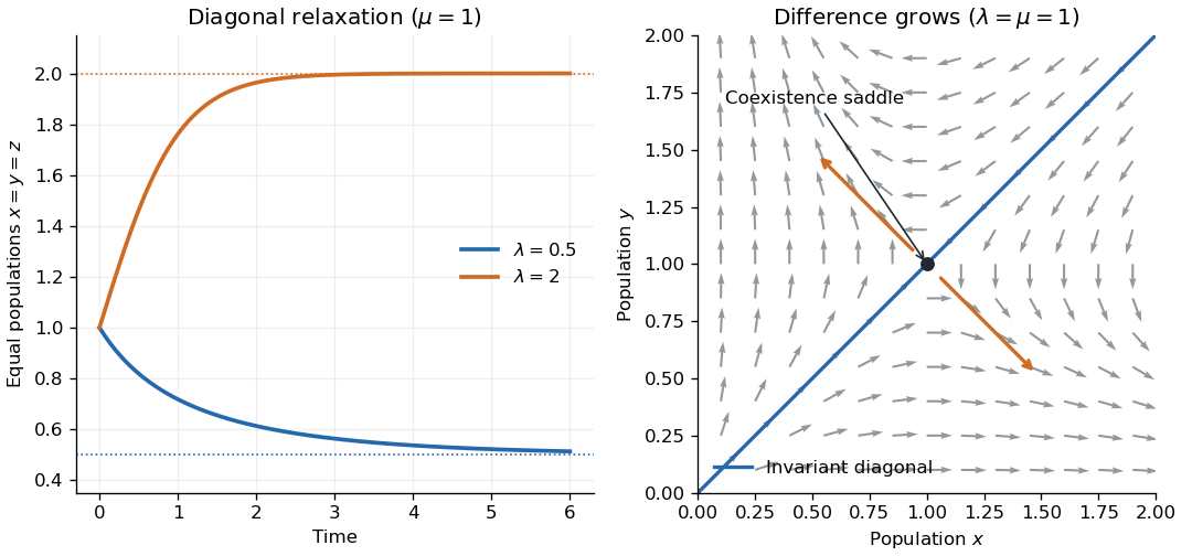
Symmetric population relaxation and transverse instability
. Details. 
For an explicit error estimate, use the martingale decomposition of a density-dependent jump process:Fix and choose . Stop at the first exit from the box . On that box, has Lipschitz constant in the supremum norm. Each coordinate of has jumps bounded by and predictable quadratic variation at mostIndeed a coordinate's positive and negative jump rates are and , and the squared jump size is . Independent jump clocks give zero cross-bracket.
The Bernstein bound for bounded-jump martingales gives, for each coordinate,The Gronwall inequality applied up to givesAn exit from the box already entails an error larger than , by the choice of , so the stopped estimate controls the event of any error on the full interval. Take and use the union bound on the two coordinates:For fixed time horizon and tolerance this is exponentially small in , proving a fluid limit. The transverse instability explains why this finite-horizon estimate should not be extrapolated to arbitrarily long times without changing its constants.
Articles by others on the same topic
There are currently no matching articles.