Let and encode the alleles at two loci on a randomly chosen population haplotype. Write , and . The linkage disequilibrium coefficient isThe determinant identity follows by substituting the marginal frequencies and . All four haplotype frequencies can be recovered asThus is precisely independence of the two allelic states. Its sign depends on which alleles are labeled one, and its possible magnitude depends on the marginal frequencies.
One other measure is squared allelic correlation. For segregating loci, , their indicator-variable covariance is , and their variances are and . HenceThis is the squared correlation, useful for measuring how well one marker predicts the other in association mapping. It is undefined if a locus is monomorphic. Linkage disequilibrium describes population haplotype frequencies; genetic linkage describes transmission within meioses. Physically linked loci can have , and population mixing can produce LD even between unlinked loci.
Across a human chromosome, neighboring single-nucleotide polymorphisms often show substantial linkage disequilibrium, while average allelic correlation tends to decline with increasing genetic distance. A new mutation starts on one ancestral haplotype; repeated genetic recombination separates it from progressively more distant markers. In an ideal randomly mating two-locus population without further mutation, migration or selection, gamete formation gives , where is the recombination fraction. The marginal allele frequencies remain fixed, soHere the prime means the next-generation value, not a separately standardized LD statistic. This simple decay explains the distance trend, rather than asserting an exact deterministic law for real finite populations.
The local pattern is heterogeneous. Many regions have haplotype blocks with strong LD and a small number of common haplotypes, separated by intervals showing more historical recombination, often recombination hotspots. A hotspot can therefore cause a rapid drop in LD between markers that are close in physical distance. Block lengths and boundaries are not uniform, perfectly sharp or independent of the population and the statistical block definition. These empirical features are documented in the HapMap data.
Population history also matters. Population bottlenecks can reduce the number of ancestral haplotypes and increase the extent of LD; population stratification or admixture can create longer-range associations, including between distant loci. Different populations can consequently have different haplotype frequencies and LD patterns at the same genomic interval. Raw also varies with allele frequency, so comparing LD across markers requires attention to the chosen measure. The typical pattern is locally strong, block-like and highly variable LD, with a broad decline over genetic distance rather than a uniform chromosome-wide decay.
Suppose a disease-risk mutation first occurs on an ancestral haplotype. Descendants carrying the risk allele initially share that surrounding haplotype. Historical genetic recombination progressively replaces the flanks while retaining the disease allele, leaving linkage disequilibrium between the causal variant and some nearby genetic markers. A noncausal marker can therefore have different allele frequencies in affected individuals and suitably chosen controls. This is the basis of association mapping.
One first tests dense markers or multi-marker haplotypes for genetic association with the disease phenotype. Strongly correlated single-nucleotide polymorphisms can be represented by tag SNPs to locate an associated region efficiently. Within that region, denser genotyping and examination of disease-associated haplotypes locate historical recombination breakpoints: segments retained across independently recombined disease-bearing chromosomes are stronger candidates for containing the causal allele. Compare affected and unaffected carriers as well, since incomplete penetrance and other risk factors can prevent a perfect haplotype-disease correspondence.
Association mapping can achieve fine resolution because it uses recombination accumulated over many generations, rather than only the few observed meioses in a present-day linkage pedigree. Resolution depends on the local recombination history: a long region of strong LD may identify a disease-associated block while leaving many variants statistically indistinguishable. Additional informative haplotypes or populations with different LD can help separate them. Conversely, very weak LD requires closer marker spacing to avoid missing the causal region.
Population stratification must be controlled by ancestry-matched comparisons, statistical adjustment or an appropriate family-based association design, since ancestry can affect both disease frequency and marker frequency. A marker association alone establishes neither causality nor identity of the disease gene; nearby correlated variants must be distinguished by further genetic and functional evidence. Use LD to detect a disease-associated ancestral segment, then use historical recombinants to narrow the causal interval. The correlation between causal variants and their surrounding haplotypes, together with the value of representative markers, is illustrated in the HapMap study.
An ancestral recombination graph, or ARG, is the directed ancestry of a sample of chromosomal segments when ancestral lineages can both coalesce and undergo genetic recombination. It records which ancestral material each lineage carries, the times of events and the recombination breakpoints. At any fixed genomic position, following only the ancestral material at that position gives a marginal phylogenetic tree. Different positions can have different trees, while sharing substantial parts of their history. The graph is acyclic in time, although its underlying undirected graph can have loops because a lineage splits backwards and its ancestors can later rejoin.
For the standard neutral, constant-size, randomly mating diploid model, measure time in generations and set , where is the recombination rate across the whole segment. The backward process is a continuous-time Markov jump process on collections of lineages carrying ancestral material:
- Each unordered pair of current lineages coalesces at rate one. The parent lineage carries the union of their ancestral material, with common ancestry recorded at overlapping positions. With lineages the total coalescence rate is . The full ARG permits a pair to merge even when its carried material is disjoint; such an event creates no merger in a local tree at that instant.
- A lineage splits into two parental lineages at a recombination breakpoint. With a uniform recombination map on a segment of normalized length one, the intensity of breakpoints along a fully ancestral lineage is per unit length. If a lineage carries only part of the segment, only cuts leaving ancestral material on both sides need be retained, giving rate , where is the span between its leftmost and rightmost ancestral positions. Material to the left goes to one parent and material to the right to the other. A gap within that span still permits a cut that separates two carried pieces.
For a state with lineages, independent exponential event clocks give total rateThe next waiting time has exponential distribution with rate ; choose its event type in proportion to the corresponding rate. A coalescing pair is uniform among unordered pairs; a recombining lineage is selected with weight and its breakpoint is uniform over its active span. With a nonuniform genetic map, use the corresponding integrated intensity and map-weighted breakpoint distribution. Initially all sample lineages span the whole segment, so the initial rate is . Ancestral material no longer needed after its sample copies have found their local common ancestor can be pruned.
Mutations are placed independently on the resulting ancestral branches, with local rate in coalescent units for a locus having scaled mutation parameter . Without recombination, the graph reduces to a single Kingman's coalescent tree. With recombination, each individual locus still has that marginal coalescent distribution, but trees at different loci are dependent. The ARG combines backward pairwise mergers with backward recombination splits; local trees are its position-specific projections. The neutral two-locus construction is developed in Hudson's two-locus model.
Five consequences of the ancestral recombination graph are:
- Linkage disequilibrium and its distance dependence. Nearby sites often inherit the same local genealogy, so mutations on their shared ancestral branches produce correlated alleles. The chance of an ancestral breakpoint between sites increases with their genetic distance, reducing shared genealogy and, on average, linkage disequilibrium. This gives the genealogical explanation of the two-locus decay calculation.
- Haplotype blocks and recombination hotspots. With a varying recombination map, the ARG has relatively few breakpoints within low-recombination regions and many near recombination hotspots. Long intervals can consequently retain a small number of common ancestral haplotypes, while genealogical relationships change more frequently across the intervening regions. This explains why LD blocks are heterogeneous rather than equally spaced units.
- Mosaic inheritance and shared ancestral tracts. Backward splits assign different pieces of one contemporary chromosome to different ancestral chromosomes. Two sampled chromosomes can therefore share a recent ancestor over one interval but not its neighbors. For a specified total of independent ancestral meioses, a tract of genetic length has approximately expected crossovers under a Poisson crossover model, so its probability of remaining intact is . This relates long IBD segments to recent common ancestry, while distinguishing tract-boundary sampling from length-biased sampling at a random genomic point.
- Incompatible site patterns and four observed gametes. Under an infinite sites mutation model on a single rooted tree, the descendant sets of two mutations are nested or disjoint. They cannot cross, so all four haplotypes cannot occur. Recombination permits different local trees: one site's derived clade can be and the other's , producing all four without repeated mutation. The four-gamete test therefore detects a failure of the unrecombined, single-mutation-per-site model. Recurrent mutation would be an alternative explanation if the infinite-sites assumption were dropped.
- Variation in local diversity and allele frequencies. Coalescent mergers describe genetic drift; their random times produce different branch lengths and descendant-group sizes. Recombination makes these genealogies vary along the chromosome. Conditional on a local genealogy, its segregating site count is Poisson with mean , so a longer tree tends to contain more variants. A mutation on a branch subtending of the samples appears at sample frequency . Together, random branch lengths, descendant counts and mutations explain heterogeneous local diversity and the distribution of allele frequencies without requiring selection.
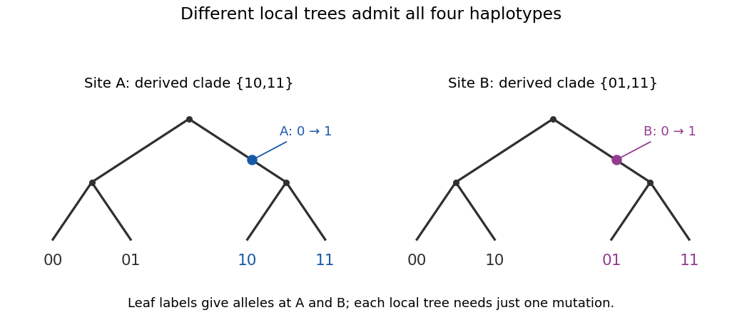
Different local genealogies can generate all four haplotypes with one mutation per site
. Details. 
Shared ancestry explains correlation; recombination makes ancestry a mosaic; mutation on the resulting branches converts genealogy into observed variation. These explanations use the neutral ARG, with a variable recombination map where stated. Selection, population subdivision or changing population size can also be studied genealogically, but require extending the event model rather than being consequences of the constant-size panmictic neutral process alone.
Articles by others on the same topic
There are currently no matching articles.