Past exam of the mathematics course of the University of Cambridge / 2005 / iii / Paper 51 / 1

A phase diagram partitions a space of thermodynamic controls into regions with distinct equilibrium phases. Its boundaries indicate phase coexistence or continuous phase transitions; a critical point is a termination of coexistence where the distinction between phases disappears. A concrete three-dimensional control space is $(T,\Delta ,h)$ for the Blume–Capel model: a spin can be $0$ or $\pm 1$, the exchange favors aligned nonzero spins, and $\Delta$ controls the energetic cost of nonzero spins. Varying $\Delta$ changes the balance between a continuous ordering transition and a first-order phase transition. Their meeting is a tricritical point.

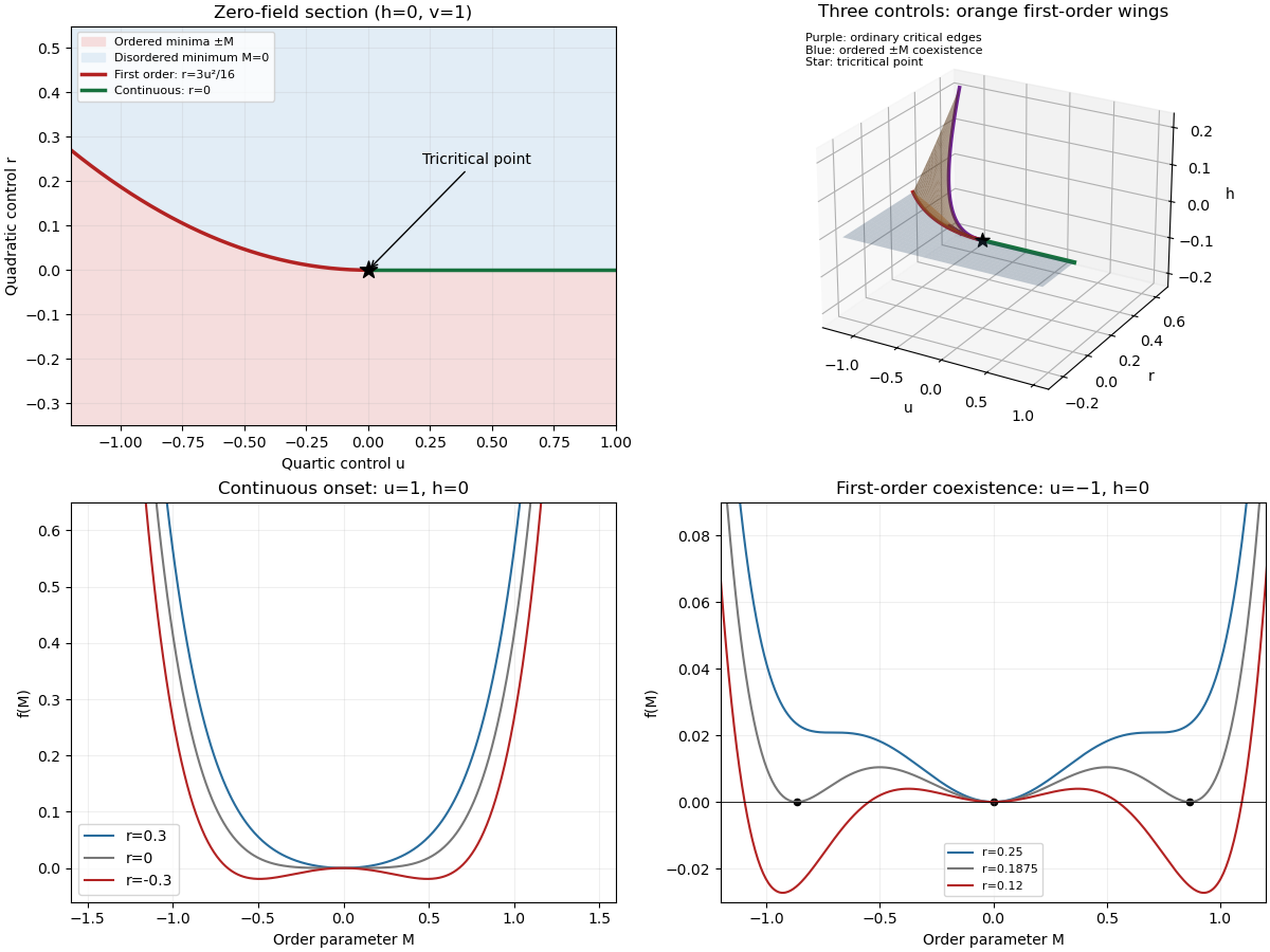
Locally, the same structure is displayed by the Landau free energywith three controls $(r,u,h)$. For $u>0$, the line $r=h=0$ consists of ordinary critical points. For $u<0$, equal free energies of $M=0$ and a nonzero stationary point requireEliminating $r$ gives the tricritical three-phase lineHere $M=0$ and both signs of $M$ coexist, with a discontinuous order parameter. Below this line, or below $r=0$ when $u>0$, the plane $h=0$ is an ordered phase coexistence sheet: crossing it reverses the sign of $M$. Two tricritical wings also extend to nonzero $h$, separating weakly and strongly magnetized states of the same sign. Their ordinary critical points satisfy $f^{\prime }=f^{\prime \prime }=f^{\prime \prime \prime }=0$. Since $f^{\prime \prime \prime }=6uM+20v{M}^3$, their tricritical wing critical edges areAt these edges $f^{\prime \prime \prime \prime }=-12u>0$, giving an ordinary quartic critical expansion around $M_c$. All these structures end at the tricritical point $r=u=h=0$. The diagrams show both the zero-field section and the genuinely three-dimensional coexistence structure.

For the final critical exponent calculation, take $r=at$ with $a>0$, $t=(T-T_c)/T_c$, and hold the other controls fixed. At an ordinary critical point, the quartic term dominates the sextic term. For $h=0$ and $r<0$,whereas on the disordered side the singular contribution is zero. Two temperature derivatives give a finite jump in heat capacity, so $\alpha =0$. At $r=0$, the equation of state is $h=u{M}^3+O(M^5)$, so $\delta =3$.

Along the tricritical trajectory $u=0$, the nonzero minimum obeys $M^4=-r/v$ andThus two temperature derivatives produce $|t{|}^{-1/2}$. At $r=u=0$, $h=v{M}^5$. Therefore the mean-field critical exponents areWith $A$ the thermodynamic free energy, the physical sign is $C=-T{\partial }_T^{2}A$, rather than the positive sign printed in the paper. This correction affects the sign of the heat capacity, not its critical exponent. The tricritical result assumes that the independent quartic control is tuned to zero; a generic trajectory through nearby ordinary critical points need not have these exponents.

An order parameter distinguishes the equilibrium phases and captures the relevant broken symmetry. For an Ising model, it is the spontaneous magnetization: its sign changes under spin reversal, and it is zero in the symmetric phase. Spontaneous magnetization means taking the thermodynamic limit before sending the external field to zero; the finite-volume zero-field mean can vanish even in an ordered phase.

In Landau-Ginzburg theory, a slowly varying real scalar field $\varphi (x)$ represents the coarse-grained local order parameter. A useful local free-energy density gives the functionalAt zero field, spin-reversal symmetry excludes odd powers. The gradient term penalizes rapid spatial variation. The field $h$ is the field conjugate to an order parameter. The mean-field approximation replaces the fluctuating scalar field by the equilibrium minimizer; a uniform minimizer has $\varphi =M$ and obeys $rM+u{M}^3+v{M}^5=h$.

In a first-order phase transition, two distinct global minima of the Landau free energy have equal values and exchange stability. The equilibrium order parameter jumps, and a first derivative of the equilibrium free energy is discontinuous. Depending on the direction through the phase diagram, that derivative can be magnetization, entropy or another conjugate quantity; a first-order transition need not have latent heat along every chosen path.

In a continuous phase transition, the equilibrium order parameter changes continuously while the curvature at the critical minimum vanishes. For $u>0$ and $h=0$, $M=0$ is stable for $r>0$, but for $r<0$ the stable minima have $M\simeq \pm \sqrt{-r/u}$. The order parameter therefore goes continuously to zero at $r=0$; the inverse magnetic susceptibility vanishes there.

For $u<0$, the sextic term stabilizes the Landau free energy. The nonzero minima can become favorable while $M=0$ still has positive curvature. At $r=3u^2/(16v)>0$ they coexist with $M=0$, so the order parameter jumps to magnitude $\sqrt{-3u/(4v)}$. Finding a stationary point alone does not locate the transition: equilibrium requires comparing the values of all competing minima. Spinodal boundaries describe loss of local stability, not coexistence.

Universality of critical phenomena means that many microscopic models approach the same long-distance renormalization-group fixed point. After repeated coarse-graining, irrelevant operators lose influence, whereas a few relevant operators describe deviations from criticality. Models with the same spatial dimension, order parameter symmetry, interaction range and appropriate relevant controls can therefore have the same universality class despite very different microscopic constituents.

The critical exponents, appropriately normalized scaling functions and certain amplitude ratios are universal. The transition temperature, individual amplitudes, microscopic length scale and analytic background in the free energy are generally nonuniversal. The numerical value assigned to an order parameter also depends on normalization. Landau-Ginzburg theory expresses this distinction by using a common symmetry-allowed functional form while allowing its coefficients to depend on the material. Computing the true critical exponents below the upper critical dimension requires retaining fluctuations, rather than merely minimizing that functional.

The relevant comparison is a short-range, uniaxial Ising ferromagnet and the liquid–gas critical point of water in three dimensions. Both have one real scalar order parameter: magnetization in the ferromagnet and the appropriately shifted density in the fluid. The magnetic field and a suitable pressure/chemical-potential combination provide the corresponding fields conjugate to an order parameter.

The fluid has no exact microscopic spin-reversal symmetry. Nevertheless, at the liquid–gas critical point the first three derivatives of the local thermodynamic potential can be eliminated or tuned by shifting the density and mixing the thermodynamic control variables. The leading stable expansion is then quartic, with the same long-distance renormalization-group fixed point as the three-dimensional short-range Ising model. The microscopic asymmetry produces corrections and analytic mixing of observables, rather than a different leading universality class.

Thus the scalar liquid–gas critical point and the short-range Ising ferromagnet share a universality class. This does not assert that every ferromagnet does: an isotropic vector-spin magnet or one dominated by long-range dipolar interactions can have different critical behavior. Nor does it identify every phase transition of water with its liquid–gas critical point.

Critical exponents describe leading singular powers as the reduced temperature $t$ or conjugate field approaches zero. With ${\beta }_m$ used for the order-parameter critical exponent to avoid confusion with inverse temperature, the definitions includeAt criticality the connected correlation function behaves as $G(r)\sim r^{-(D-2+\eta )}$. These definitions refer to the singular part and allow additional logarithms at marginal dimensions.

For an ordinary scalar Landau free energy, the equation of state is $h=rM+u{M}^3$. Below the transition $M^2=-r/u$, giving ${\beta }_m=1/2$. Differentiating the equation of state gives ${\chi }^{-1}=r+3u{M}^2$: it equals $r$ above and $-2r$ below the transition, so $\gamma =1$. The quadratic fluctuation kernel is $\kappa k^2+r$ in the symmetric phase, giving correlation length $\xi =\sqrt{\kappa /r}$ and $\nu =1/2$. At zero mass the momentum-space correlation function is proportional to $k^{-2}$, so $\eta =0$. The minimized free energy and critical equation of state give $\alpha =0$ and $\delta =3$, as calculated in the root solution.

At the tricritical point, $u=0$ and $h=rM+v{M}^5$. Then $M\sim (-r{)}^{1/4}$, and ${\chi }^{-1}=r+5v{M}^4$ is $r$ above and $-4r$ below the transition. The gradient kernel still gives $\nu =1/2$ and $\eta =0$. ThereforeThese are mean-field critical exponents. A systematic derivation incorporating fluctuations uses the renormalization group, extracts the relevant scaling eigenvalues, and differentiates the singular free-energy density, as in Question 3.

A tricritical point requires two independent even coefficients in the Landau free energy to vanish: $r=u=0$, with $v>0$ providing stability. At $h=0$, the ordinary critical line $r=0,u>0$ meets the tricritical three-phase line $r=3u^2/(16v),u<0$. The order parameter discontinuity along the first-order line is $\sqrt{-3u/(4v)}$, which goes to zero at their meeting.

The positive sextic coefficient makes this a different leading local potential from an ordinary quartic critical point. Consequently its mean-field critical exponents, crossover behavior and upper critical dimension differ. There are two relevant even tuning directions near the tricritical point, in addition to the conjugate odd field. The root solution and labelled phase diagram display the three controls and the tricritical wings; varying $h$ can give a first-order reversal within the ordered coexistence sheet, a first-order weak/strong transition on a wing, or a continuous transition at a wing's ordinary critical edge.

The upper critical dimension is the dimension at which the leading nonlinear interaction is marginal under Gaussian scale transformations. Normalize the gradient term and rescale $x=b{x}^{\prime }$ so that $\varphi (x)=b^{-(D-2)/2}{\varphi }^{\prime }(x^{\prime })$. A coupling $g_{2p}\int {\varphi }^{2p}{d}^{D}x$ then scales byThusBelow this dimension, the interaction is a relevant operator at the Gaussian fixed point, so neglecting long-wavelength fluctuations is not self-consistent near criticality. A direct Ginzburg criterion gives the same result: the fluctuation in a correlation volume scales as $⟨(\delta \varphi {)}^2{⟩}_{\xi }\sim {\xi }^{2-D}$. For ordinary ordering $M^2\sim r/u\sim {\xi }^{-2}/u$, their ratio is proportional to $u{\xi }^{4-D}$. Along a tricritical trajectory $M^2\sim (|r|/v{)}^{1/2}\sim {\xi }^{-1}/\sqrt{v}$, giving ratio proportional to $\sqrt{v}{\xi }^{3-D}$. These ratios grow without bound below the corresponding upper critical dimension.

At $D=D_c$, the interaction is marginal. Mean-field powers can survive, but acquire multiplicative logarithmic corrections; it is too strong to say that all mean-field exponent values necessarily fail at equality. Above $D_c$, fluctuations do not change the leading mean-field critical exponents, although a dangerously irrelevant coupling can invalidate naive hyperscaling.