Past exam of the mathematics course of the University of Cambridge / 2006 / iii / Paper 41 (Applied Statistics)

Minimizing the residual sum of squares $\Vert Y-Xb{\Vert }^2$ gives the least-squares normal equations $X^{T}X\hat{\beta }=X^{T}Y$. Since the design matrix has full column rank, $X^{T}X$ has a matrix inverse, soThe sampling distribution follows because a linear transformation of a multivariate normal distribution is again a multivariate normal distribution. Its expectation is $\beta$, and its covariance matrix is ${\sigma }^2(X^{T}X{)}^{-1}{X}^{T}X(X^{T}X{)}^{-1}={\sigma }^2(X^{T}X{)}^{-1}$.

The hat matrix is $H=X(X^{T}X{)}^{-1}{X}^T$. It is the orthogonal projection matrix onto the column space of $X$: $H^T=H$, $H^2=H$ and $HX=X$. Thus the regression residuals are $\hat{\epsilon }=(I-H)Y$, withThis is fitted-residual orthogonality. The vectors are jointly normal, so independence of uncorrelated jointly normal variables strengthens both zero-covariance statements to independence.

For the quadratic linear regression, the columns of the design matrix are $1,x,x^2$. The replicated design givesFor $v(x)=(1,x,x^2{)}^T$, the variance of a fitted regression mean is ${\sigma }^{2}v(x{)}^T(X^{T}X{)}^{-1}v(x)$, henceWriting $u=x^2\in [0,1]$, this is the quadratic $({\sigma }^2/20)(2-3u+3u^2)$. Its derivative vanishes at $u=1/2$; it decreases before that point and increases afterwards. Therefore the maximum is ${\sigma }^2/10$ at $x=-1,0,1$, and the minimum is ${\sigma }^2/16$ at $x=\pm 1/\sqrt{2}$.

At $100^{\circ }\mathrm{C}$, $x=0$ and the expected yield is $\alpha$. The unbiased residual variance estimate is $s^2=2.43/(30-3)=0.09$. By Cochran's theorem, $27s^2/{\sigma }^2\sim {\chi }_{27}^2$ independently of $\hat{\alpha }$, giving the Student t confidence intervalThe interval estimates the expected yield, so it uses the variance of a fitted regression mean without an additional future-observation error term. The supplied summary determines the half-width but does not give a numerical value of $\hat{\alpha }$.

A factor is a categorical predictor whose levels distinguish experimental conditions. Two factors have a statistical interaction when the effect of changing one depends on the other's level. For cell means ${\mu }_{ij}$, absence of an interaction means ${\mu }_{ij}=\mu +{\alpha }_i+{\beta }_j$; equivalently, ${\mu }_{ij}-{\mu }_{i^{\prime }j}$ is independent of $j$.

Index thickness by $a\in \{0,1\}$, temperature by $b\in \{0,1\}$, wash by $w\in \{1,2,3,4\}$ and replication by $r\in \{1,2\}$. The full factorial design has the normal linear modelThe errors are independent with a common positive variance. Sum-to-zero constraints in each factor index, or the displayed treatment coding, identify the mean coefficients. This full model allows an arbitrary mean in each of the sixteen cells.

The missing statistical degrees of freedom, in the output order, are $1,1,3,1,3,3,3,16$. The first seven entries total fifteen; with the regression intercept there are sixteen mean coefficients among thirty-two observations, leaving sixteen residual statistical degrees of freedom. Balanced factorial orthogonality makes the term sums of squares in ANOVA independent of their ordering.

All terms involving wash have nonsignificant individual F-tests, and it is useful to test their removal jointly. The reduced model omits twelve mean coefficients. Its residual sum of squares is $57.09875$, compared with $32.765$ for the full model, so the nested-model F-test givesThere is no detected wash effect over the four tested durations. Removing its main effect and all its interaction terms respects the principle of marginality. Retaining the very large thickness-by-temperature interaction is essential: the thickness effect changes substantially with temperature.

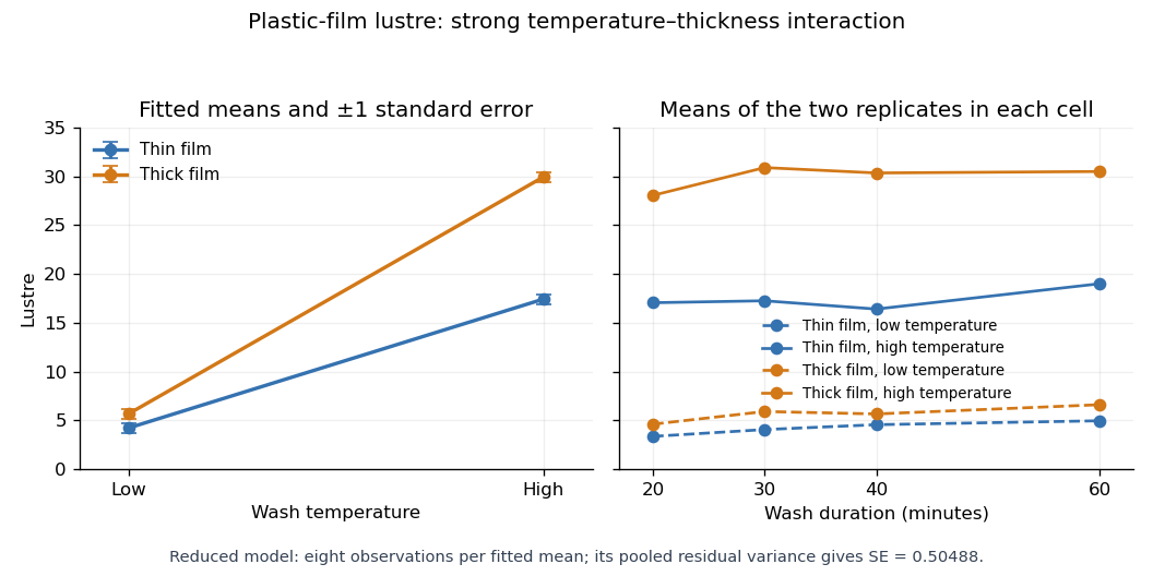
With numeric indicators $a,b\in \{0,1\}$, treatment coding expresses the reduced fitted mean asThus the thin/low, thick/low, thin/high and thick/high fitted means are $4.225,5.6875,17.425,29.950$, respectively, at every wash level. Each is the sample mean of eight observations. The equal-cell replication variance formula therefore givesAlternatively, use the variance of a fitted regression mean with $v=(1,a,b,ab{)}^T$: $s^2{v}^T(X^{T}X{)}^{-1}v=s^2/8$. Individual coefficient standard errors cannot simply be added; their covariances enter the fitted-mean calculation.

Increasing temperature raises fitted lustre by $13.2$ for thin film and $24.2625$ for thick film. Increasing thickness raises it by $1.4625$ at low temperature and $12.525$ at high temperature. Their difference, $11.0625$, is the estimated interaction contrast; its standard error is $1.0098$, giving $t\simeq 10.956$ on twenty-eight statistical degrees of freedom. The interaction plot shows this strong departure from parallel mean lines, while the wash panel shows the much smaller variation across wash durations. Neither the nonsignificant wash test nor the plot proves that its true effect is exactly zero.

The Poisson distribution mass function isIt is an exponential dispersion family of order one withIndeed, $b^{\prime }(\theta )=e^{\theta }=E(Y)$ and $\varphi b^{\prime \prime }(\theta )=e^{\theta }=\mathrm{Var}(Y)$. A generalized linear model specifies independent random variables from a response exponential family, together with a linear predictor and a link function relating it to the response mean. The Poisson canonical link is $g(\mu )=\log \mu$.

For the insurance counts, let class $1$ and merit $0$ be the reference levels in a regression factor. The fitted Poisson regression assumesThe insured exposure $n_{ij}$ is known; its logarithm is an offset, not a coefficient to estimate. The model has eight free mean parameters and fixes the dispersion parameter at one. It assumes additive class and merit effects on the log-rate scale, hence multiplicative effects on the rate scale without a class-by-merit interaction.

Apart from constants independent of the parameters, the log-likelihood isDifferentiating gives the Poisson regression margin-matching score equationsThus the fitted totals equal the observed totals in each class and merit category, including the reference categories by subtraction. In design matrix notation these equations are $Z^T(Y-\hat{\mu })=0$. Fisher scoring solves them iteratively; the reported three iterations describe the numerical fit, not an additional statistical result.

The regression intercept gives the baseline fitted claim rate $e^{-2.0357359}=0.130584$ per insured car year. The merit rate ratios, relative to merit $0$ at the same class, areThe class rate ratios, relative to class $1$ at the same merit, areEach predicted cell rate is the baseline rate times its class and merit multipliers. The output's coefficient-to-standard error ratios are asymptotic normal Wald test statistics under the fitted Poisson regression, despite the software label “t value”; there is no estimated Gaussian residual scale in this model. All nonreference effects have very large absolute ratios.

The null Poisson deviance is $33854.16$ on nineteen statistical degrees of freedom; adding the seven factor coefficients reduces it by $33274.6437$. But the final Poisson deviance is still $579.5163$ on twelve statistical degrees of freedom, and the deviance residuals include values near $-10.79$ and $11.63$. These are far beyond what a well-fitting unit-dispersion model would normally produce. The additive Poisson model fits substantially better than a common rate, but remains grossly inadequate. A class-by-merit interaction, overdispersion, or statistical dependence between claims could contribute; the summary alone does not distinguish these explanations. Its very small nominal standard errors and formal Wald tests rely on the rejected model, so improved mean structure and error assumptions are needed before treating them as reliable uncertainty assessments.

For independent binomial distributions, the log-likelihood, up to known binomial coefficients, isThe saturated statistical model maximizes each term at ${\tilde{p}}_i=y_i/n_i$. Under the logit link, the fitted probabilities are ${\hat{p}}_i=(1+e^{-x_i^T\hat{\beta }}{)}^{-1}$. Subtracting the fitted log-likelihood from the saturated log-likelihood gives the binomial devianceA zero-count summand uses the continuous convention $0\log 0=0$. For the restricted model, replace ${\hat{p}}_i$ by ${\hat{p}}_i^{(0)}=(1+e^{-{\tilde{x}}_i^T\hat{\tilde{\beta }}}{)}^{-1}$ to obtain $D_0$. Since the saturated likelihood cancels, $D_0-D_1=2({\hat{\ell }}_1-{\hat{\ell }}_0)$ is the likelihood-ratio test statistic. For the nested restriction setting $p-k$ coefficients to zero, Wilks theorem gives the asymptotic chi-squared distribution ${\chi }_{p-k}^2$ under regularity and an interior true parameter; reject for a large difference.

For the six anther cells, ${\omega }_0$ gives a common success probability, ${\omega }_1$ gives a separate probability for each storage condition, ${\omega }_2$ gives a common intercept and a log-force slope, and ${\omega }_3$ gives storage-specific intercepts with a common log-force slope. Their parameter counts are $1,2,2,3$, so their residual statistical degrees of freedom are $5,4,4,3$. In ${\omega }_3$, storage has a constant effect on log odds; multiplying force by $r$ multiplies the odds by $r^{\beta }$ in either storage group.

The relevant nested likelihood-ratio tests at the $5\%$ level are:

The two two-parameter models ${\omega }_1$ and ${\omega }_2$ are not nested, so their deviance difference has no ordinary nested chi-squared distribution calibration. The preferred parsimonious model is ${\omega }_1$, with a storage effect and no log-force effect. Its deviance goodness-of-fit test is acceptable: $D_1=5.173<9.49$ on four statistical degrees of freedom. The common-probability model also passes its separate goodness-of-fit comparison, $10.452<11.07$, but this does not contradict the relative evidence for adding storage: the two tests assess different null hypotheses. These are large-sample approximations; sufficiently large expected successes and failures, not merely the number of anthers, underpin their calibration.

Let $X$ denote the observed data, $Z$ the unobserved data and $\theta$ the model parameters. The expectation-maximization algorithm works with the complete-data log-likelihood ${\ell }_c(\theta ;X,Z)$. Given ${\theta }^{(r)}$, its E-step computeswhere the conditional expectation uses the old parameter, while $\theta$ remains the argument to maximize. Its M-step chooses ${\theta }^{(r+1)}$ maximizing this function over the parameter space. EM likelihood monotonicity ensures that an M-step increasing $Q$ cannot decrease the observed-data log-likelihood. It does not guarantee a global maximum, so convergence and any parameter constraints must still be checked.

The sum of the two independent exponential times has a hypoexponential distribution. By convolution of probability densities, for $t>0$ and $d={\lambda }_1-{\lambda }_2>0$,Thereforeand $g(t)=0$ for $t<0$. This is a nonnegative normalized probability density function. At the equal-rate boundary it tends to ${\lambda }^{2}t{e}^{-\lambda t}$, a shape-two Gamma distribution.

Put $A={\sum }_{i=1}^3{S}_{i1}$, $B={\sum }_{i=1}^3{S}_{i2}$ and $d={\lambda }_1-{\lambda }_2$. Independence of the pairs makes their likelihood contributions multiply. The three fully observed pairs contribute $({\lambda }_1{\lambda }_2{)}^3{e}^{-{\lambda }_{1}A-{\lambda }_{2}B}$; each remaining pair contributes its hypoexponential distribution density. Thus the observed-data log-likelihood isAn equivalent expression, convenient for calculations, isThe apparent singularity as $d\downarrow 0$ cancels between the last sum and $-5\log d$. The resulting equal-rate limit is finite for positive observed times.

Take the missing strong-swimmer times $U_j=S_{j1}$, $j=4,\dots ,8$, as the latent variables. Their partners' times are $T_j-U_j$. The complete-data log-likelihood isFor the E-step of the expectation-maximization algorithm, use the conditional split of two exponential times. At the old rates, with $d_r={\lambda }_1^{(r)}-{\lambda }_2^{(r)}>0$,This is a truncated exponential distribution, whose conditional expectation isThe displayed mean follows by integrating $u{e}^{-d_{r}u}$ against the conditional density; the missing weak-swimmer mean is $T_j-m_j^{(r)}$. As $d_r\to 0$, the conditional density becomes uniform on $(0,T_j)$ and $m_j^{(r)}\to T_j/2$.

Write $U_r=A+{\sum }_j{m}_j^{(r)}$ and $V_r=B+{\sum }_j(T_j-m_j^{(r)})$. The E-step objective isSetting its partial derivatives to zero gives the unconstrained M-stepThese are eight divided by the completed expected totals for the corresponding swimmers; imputing only observed pair totals without the conditional split would not perform the E-step.

The stated ordering must also be enforced. The ordered-rate exponential M-step accepts these updates when $U_r<V_r$, so ${\lambda }_1^{(r+1)}>{\lambda }_2^{(r+1)}$. Otherwise its maximum on the closed constraint ${\lambda }_1\ge {\lambda }_2$ lies atUnder a strictly open constraint ${\lambda }_1>{\lambda }_2$, a boundary optimum is only a supremum; a finite interior maximizer is not assured for every possible sample. One should report that situation rather than swap the labeled swimmer groups. Starting from positive ordered rates, iterate the E-step and constrained M-step until the parameter changes and observed log-likelihood improvement are small. EM likelihood monotonicity applies to every exact constrained M-step. No numerical swimming times are supplied, so the data-dependent updates, rather than fabricated numerical estimates, are the answer.