Past exam of the mathematics course of the University of Cambridge / 2007 / iii / Paper 43 (Applied Statistics)

This is an analysis of covariance: achievement is the response, aptitude is a quantitative covariate, and teaching method is a categorical explanatory variable. The usual normal linear model assumes independent errors with common variance ${\sigma }^2$.

read.table reads the data with a header row; attach makes its columns directly accessible, and the two printed vectors confirm their ordering. rep(1:3, each=7) supplies the three group labels, and factor makes them categorical. The contrast option selects treatment coding for unordered factors, with method A as the first-level reference. The polynomial option would apply to ordered factors and has no role here.

The formula using aptitude * Group includes both main effects and their interaction. Writing $I_B,I_C$ for the method indicators, its fitted mean has the formThus A, B and C have separate intercepts and slopes. There are six coefficients and $21-6=15$ residual statistical degrees of freedom. The analysis of variance table uses sequential sums of squares: adding aptitude to an intercept-only model removes $36.57548$ from the residual sum of squares; subsequently adding the two group indicators removes $16.93200$; adding the two slope interactions removes only $0.66714$. The remaining sum of squares is $9.63490$, giving mean square $9.63490/15=0.64233$.

Each displayed F-test divides the added term's sum of squares by its statistical degrees of freedom and then by this full-model residual mean square. In particular the interaction test isThere is no evidence that the slopes differ, so the common-slope model is preferable among the fitted models. The small group $p$-value concerns differences after including aptitude, whereas the first aptitude row is sequential and does not adjust for Group. It should not be interpreted as the covariate test after treatment adjustment.

The additive formula gives the parallel-lines modelIt has four coefficients and $17$ residual statistical degrees of freedom. Removing the interaction raises the residual sum of squares to $9.63490+0.66714=10.30204$, but lowers the residual mean square to $10.30204/17=0.60600$. The sequential aptitude and group sums of squares are unchanged. The adjusted group test is now $F=(16.93200/2)/0.60600=13.97024$ on $(2,17)$ statistical degrees of freedom, with $p=0.0002579$: after allowing for initial aptitude, the methods are not all equally effective.

summary(..., cor=F) displays the fitted coefficients, their standard errors, the individual $t$ statistics, and two-sided $p$-values; it omits the coefficient-correlation matrix. The intercept $2.8367$ is the fitted A mean at aptitude zero, which is outside the observed range and is mainly a parametrization device. The common slope $0.7429$ predicts about $0.74$ extra achievement units per aptitude unit, holding method fixed. Its adjusted $t$ test is $5.2267$ on $17$ statistical degrees of freedom, with $p$ about $0.0001$. The method coefficients are adjusted differences from A, not the B and C intercepts themselves. The three fitted lines areThe B-minus-A estimate is $2.1878$ with standard error $0.4545$ and $t=4.8139$; the C-minus-A estimate is $1.8612$ with standard error $0.4240$ and $t=4.3901$. Both comparisons are strongly significant.

The B-minus-C comparison needs its own treatment contrast; its significance cannot be read off either comparison with A. Reconstructing the coefficient covariance from the design givesThus there is no detectable difference between B and C. This is consistent with pooling their effects in a further reduced model, but does not establish exact equality.

The residual standard error is $\sqrt{0.60600}=0.7785$. The five-number residual summary shows deviations on both sides of zero, with the largest magnitude about $1.74$; it does not by itself verify constant variance or normality. The coefficient of determination $R^2=0.8386$ means about $84\%$ of the achievement variation about its overall mean is explained. The overall $F=29.43$ compares all three nonintercept coefficients with zero, on $(3,17)$ statistical degrees of freedom; its $p$-value is $5.889\times 10^{-7}$. Printed coefficient $p$-values rounded to 0.0000 are small, not literally zero.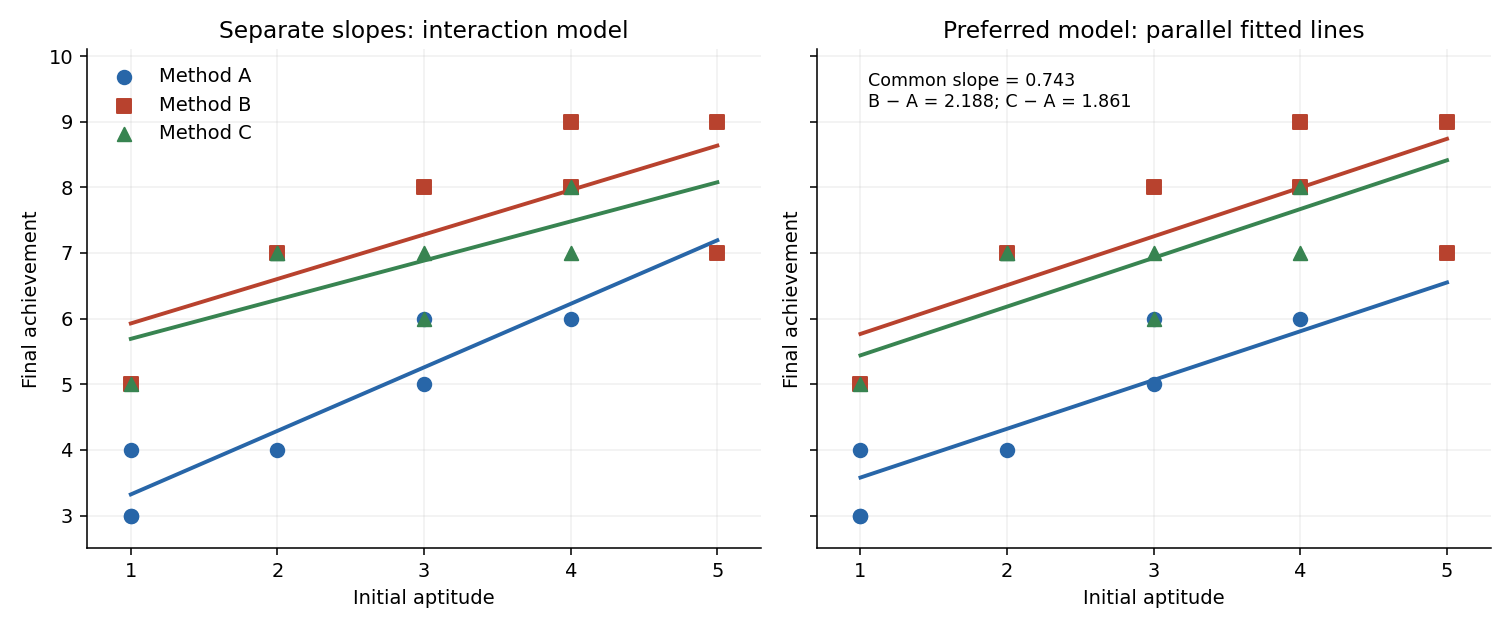

The following original sketch shows the separate-slope model and the preferred parallel-line fit.

At the same initial aptitude, B and C give higher predicted achievement than A, with no convincing difference between B and C. Interpreting this adjusted association as a causal teaching effect additionally relies on the experimental allocation and error assumptions.

For an exponential dispersion family, differentiating the normalization integral with respect to $\theta$ gives an expected score of zero. The score is $(Y-b^{\prime }(\theta ))/\varphi$, hence $E(Y)=b^{\prime }(\theta )$. Differentiating again, the expected squared score is $b^{\prime \prime }(\theta )/\varphi$; it is also $\mathrm{Var}(Y)/{\varphi }^2$. ThusThe canonical link function sets the linear predictor equal to the natural parameter: $g(\mu )=\theta =(b^{\prime }{)}^{-1}(\mu )$. The variance function is $V(\mu )=b^{\prime \prime }((b^{\prime }{)}^{-1}(\mu ))$, so $\mathrm{Var}(Y_i)=\varphi V({\mu }_i)$; the dispersion parameter $\varphi$ is separated from the mean-dependent factor.

The saturated statistical model has a separate mean for each response and fits ${\tilde{\mu }}_i=y_i$, with boundary parameters interpreted by limits. At the same fixed dispersion, its log likelihood and the fitted model's log-likelihood define the scaled devianceThe unscaled deviance isKeeping dispersion fixed in this definition is essential; it is not a comparison with a separately estimated zero variance in a Gaussian saturated fit.

For the normal distribution, expanding its density exponent givesConsequentlyHere $V(\mu )=1$ and the canonical link is the identity, so ${\mu }_i={\beta }^T{x}_i$. The saturated natural parameter is ${\tilde{\theta }}_i=y_i$. Substitution into the deviance formula yields

For the cholesterol fits, all formulae include an intercept. Model 1 has age and BMI with three coefficients; models 2 and 3 have one of these covariates with two coefficients; model 4 has only the intercept. Their residual statistical degrees of freedom are respectively $27,28,28,29$. Their reported deviances are residual sums of squares, because these are Gaussian linear models.

The relevant hypothesis is $H_0:{\beta }_{\mathrm{BMI}}=0$ in the full model, against $H_1:{\beta }_{\mathrm{BMI}}\ne 0$, with age already present. Thus compare model 2 with model 1 using the partial F-test. Its extra sum of squares is $31.64-27.10=4.54$, and the common variance is estimated from model 1 by ${\hat{\sigma }}^2=27.10/27$. ThereforeSince $4.52325>4.210$, reject at $5\%$; the two-sided coefficient-test equivalent has $p\simeq 0.0427$. BMI is associated with cholesterol after adjustment for age, under the linear Gaussian model. The RSS values alone do not identify the sign of its coefficient or the size of the association.

For comparison, the marginal BMI test would compare model 4 with model 3, giving $F=13.88/(35.82/28)=10.8498$ on $(1,28)$ statistical degrees of freedom, with $p\simeq 0.00268$. This does not answer the adjusted question and makes the BMI evidence appear stronger than the conditional test. Age also contributes after BMI: comparing model 3 with model 1 gives $F=8.72/(27.10/27)=8.6878$ on $(1,27)$ statistical degrees of freedom, with $p\simeq 0.00653$. Thus retaining both predictors is supported at the stated level.

A raw deviance difference must not simply be compared with the supplied ${\chi }_1^2$ cutoff: Gaussian dispersion is unknown and the differences here are unscaled. If ${\sigma }^2$ were known, the scaled difference $4.54/{\sigma }^2$ would have a ${\chi }_1^2$ law. Estimating it from the full fit gives the exact finite-sample $F$ comparison above, with the appropriate denominator statistical degrees of freedom.

The logit link makes the probability constant within each group: write $p_i=\{1+\exp [-(\mu +{\alpha }_i)]{\}}^{-1}$, with ${\alpha }_1=0$. Let $S_i={\sum }_{j=1}^k{Y}_{ij}$ and $N=km$. Independence gives $S_i\sim \mathrm{Bin}(N,p_i)$. Up to terms independent of the parameters, the log likelihood isThe likelihood equations areTogether they also imply $S_1-N{\hat{p}}_1=0$. Thus, when all totals satisfy $0<S_i<N$,The group logits are unconstrained apart from their parametrization, and each binomial log likelihood is strictly concave in its logit, so these equations give the unique finite maximum. A total of $0$ or $N$ instead gives a boundary probability and an infinite logit; a finite MLE need not exist in that case.

For $n=2$, keep $0<p_1,p_2<1$ fixed and let $N=km\to \infty$. Since ${\hat{p}}_1=S_1/N$, the central limit theorem gives $\sqrt{N}({\hat{p}}_1-p_1)\stackrel{d}{\to }N(0,p_1(1-p_1))$. The derivative of the logit is $1/[p_1(1-p_1)]$, so the delta method gives the baseline logit estimator in a group-factor binomial model lawThe second group does not improve the baseline estimate because it has its own free offset. Equivalently, the Fisher information matrix for $(\mu ,{\alpha }_2)$ isIts first diagonal entry confirms the same asymptotic variance.

factor(day) treats the nine days as categorical rather than imposing a numerical time trend. rep(400,27) supplies the number of trials for every dish, and prop is the observed surviving proportion. The contrast setting uses treatment coding with day 1 as reference; the ordered-factor polynomial option is unused. Supplying these proportions to glm with the binomial family and weights $400$ gives precisely the grouped-binomial logistic regression likelihood for the counts. The weights represent trial counts, not additional independent dish observations. The binomial family's default link is the logit link and its dispersion is fixed at $1$.

Let $Y_{ij}$ be survivors in dish $j=1,2,3$ on day $i=1,\dots ,9$. Both fitted models assume independent $Y_{ij}\sim \mathrm{Bin}(400,p_i)$. Model 1 specifiesso it has one common probability and one fitted coefficient. Its estimated probability is the total surviving count divided by the total trial count, $\hat{p}=3539/10800\simeq 0.327685$.

Model 2 specifiesIt has nine coefficients and allows a separate probability for each day, while retaining a common probability for the three dishes within that day. The MLEs are the day totals divided by $1200$. In day order they areThe intercept is the first day's logit, and each other coefficient is its day's logit minus that reference. These are additive effects on log odds, not additive changes in survival probability.

The analysis of deviance adds the eight day indicators after an intercept-only model. Its residual deviance compares a fitted model with the saturated statistical model assigning one separate probability to each of the $27$ dishes. For fitted dish probabilities ${\hat{p}}_{ij}$, the binomial deviance isThe binomial scale is one, so this is also scaled deviance. The reported decrease measures the extra fit provided by day. There are $27$ observational units for these residual statistical degrees of freedom, not $10800$ separately fitted Bernoulli responses.

The null model uses one parameter, the day model uses nine, and there are $27$ grouped observations. The four missing entries, in their table order, are thereforeThe test of no day effect is $H_0:{\alpha }_2=\cdots ={\alpha }_9=0$. The nominal binomial likelihood-ratio test statistic is $\Delta D=462.8363$, compared asymptotically with ${\chi }_8^2$. Its nominal $p$-value is about $6.6\times 10^{-95}$, so the common-probability model is decisively inadequate relative to the day model. The fitted probabilities in (i) show substantial differences between days, with days 1 and 7 much higher than days 3 and 8.

However, relative improvement does not establish absolute fit. The day model's deviance goodness-of-fit test compares $D=32.7945$ with ${\chi }_{18}^2$, giving $p\simeq 0.0177$. The counts are large enough for this approximation to be reasonable. Thus at $5\%$ the day-specific binomial model still shows lack of fit. Among the two printed models it is preferred, but it should not be regarded as a fully satisfactory final model.

The residual scale estimate $D/18\simeq 1.822$ suggests overdispersion. Directly computing the Pearson statistic from the day means givesThis corroborates extra dish variation rather than the nominal binomial variance. Dish heterogeneity or dependence among cells in a dish can produce such variation. Residual checks and a quasibinomial regression or an explicit model for dish heterogeneity are sensible refinements. Allowing dispersion of this moderate magnitude would enlarge standard errors but would not plausibly remove the very large day effect. Retain day effects, while accounting for the remaining extra-binomial variation.

The experimental unit for comparing the treatments is the pot: its two plants form a pair. Let $D_i=C_i-S_i$ be cross-fertilised minus self-fertilised height in pot $i$, for $i=1,\dots ,15$. The paired Wilcoxon signed-rank test assumes independent differences with a continuous distribution symmetric about a location $\delta$. Its null is $\delta =0$, with the one-sided formulation $\delta \le 0$, against $\delta >0$. Under this location model it asks whether cross-fertilisation produces a positive shift within a pot. The location is a median, and also a mean if it exists; a hypothesis merely about a median without symmetry does not justify the signed-rank null distribution.

Test 1 uses this paired test and its exact distribution. Form the fifteen differences, omit any zero differences, rank their absolute values, and sum the statistical ranks belonging to positive differences. That positive-rank sum is the reported $V=96$. Tied absolute differences receive average statistical ranks. Under the symmetric zero-location null, conditional on their magnitudes, the signs are independent fair signs. The exact upper-tail probability is obtained from all sign allocations to the observed statistical ranks: with fifteen nonzero differences there are $2^{15}$ equiprobable allocations. For untied absolute differences the rank weights are $1,\dots ,15$; ties would require the corresponding conditional rank weights. The reported probability of a positive-rank sum at least as large as observed is $0.0206$. No normal approximation is used.

Test 2 makes exactly the same paired comparison and has the same null and alternative hypotheses. exact=F replaces the exact distribution by a normal approximation with a continuity correction. Under an untied null the positive-rank sum hasMore generally, conditional on the nonzero absolute statistical ranks $r_i$, its variance is $\frac{1}{4}{\sum }_i{r}_i^2$. The upper-tail correction places the boundary half a lattice unit below the observed statistic. Standardizing gives the reported $Z=2.0163$, and its approximate $p$-value is $1-\Phi (Z)=0.0219$. Thus the slight difference from Test 1 reflects approximation, not a different scientific question.

Test 3 omits paired=T, so it is the unpaired Wilcoxon rank sum test. Its usual distribution-free null is that two independent samples have the same continuous distribution. In a common-shape location model this is a zero location difference, against a positive cross-minus-self shift. More generally “greater” directs the test towards the cross distribution being shifted upwards; it does not turn the test into a general comparison of means or medians for arbitrary unequal shapes.

To form its statistic, pool the thirty heights, rank them together with averaged statistical ranks for ties, and add the cross-group statistical ranks to get $R_C$. Equivalently use $U=R_C-n_C(n_C+1)/2$. Under independent untied samples,If the pooled ties have sizes $t_h$ and $N=n_C+n_S$, the variance becomesSubtract the null mean and the upper-tail continuity correction, then divide by this null standard deviation. This procedure gives the reported rank-sum $Z=3.0105$. Its approximate one-sided probability is $1-\Phi (Z)=0.0013$. This describes how the statistic and probability are obtained without reconstructing the unprinted heights.

For the statistician, use the paired analysis, preferably the exact Test 1 for these fifteen pairs. The independent units are the pots, while the two heights within a pot share growing conditions and cannot be treated as independent samples. Test 2 is a reasonable approximation to the same paired test and agrees closely. Test 3 discards the matching and uses a null variance that assumes independence between the samples, so its smaller $p$-value is not a reason to prefer it. The appropriate paired result gives evidence at $5\%$, but not at $1\%$, that cross-fertilised plants have a positive height shift relative to their paired self-fertilised plants, subject to the symmetry assumption for differences.

A Gaussian generalised additive model with the identity link specifiesThe $f_j$ are unknown smooth functions estimated from the data, rather than necessarily straight lines. The model is additive in their effects, so it does not automatically contain interactions between covariates. To identify the intercept separately from the smooths, impose a constraint such as ${\sum }_i{f}_j(x_{ij})=0$ for each $j$. Linear terms can also be included alongside smooth terms. More generally a specified link function can make $g(E(Y_i))$ additive; for the normal identity-link model the mean itself has the displayed form. Smoothness is typically controlled through a basis and a roughness penalty, preventing an unrestricted smooth from interpolating all the noise.

A natural cubic spline interpolant $s$ satisfies $s(x_i)=y_i$, is twice continuously differentiable, and is a polynomial of degree at most three on each interval $[x_i,x_{i+1}]$. Its natural boundary conditions areIf defined outside the data interval, it continues linearly on both exterior intervals. Thus function values and the first two derivatives match at the knots, but the third derivative may jump.

For an explicit construction, let $h_i=x_{i+1}-x_i>0$ and $M_i=s^{\prime \prime }(x_i)$. Set $M_1=M_n=0$ and solveOn $[x_i,x_{i+1}]$, putThis formula interpolates the values and matches second derivatives; the tridiagonal equations enforce first-derivative matching. The homogeneous system has only the zero solution: in a row with maximal nonzero $|M_i|$, its diagonal coefficient strictly exceeds the sum of its neighbour coefficients, making cancellation impossible. Thus the natural interpolant exists uniquely.

With the convention that the residual term is a sum rather than an average, the penalised least squares criterion isMinimize over functions whose first derivative is absolutely continuous and whose second derivative is square-integrable, that is, the usual Sobolev space $H^2[x_1,x_n]$. The cubic smoothing spline ${\hat{g}}_{\lambda }$ is its minimizer, with natural boundary conditions and linear continuation outside the data range. It is a natural cubic spline with possible knots at the observed $x_i$, but usually does not interpolate the noisy $y_i$.

To see why the minimizer is a natural spline, for any $g$ take the natural cubic spline interpolant $s$ through its values $g(x_i)$ and write $h=g-s$. Then $h(x_i)=0$. Integrating $\int s^{\prime \prime }{h}^{\prime \prime }$ by parts on every knot interval twice gives zero: the terms involving $h$ vanish at knots, the terms involving $h^{\prime }$ cancel because $s^{\prime \prime }$ is continuous there, and the outer terms vanish by the natural boundary conditions. Hencewhile their residual sums of squares agree. Replacing $g$ by $s$ never increases the criterion. This proves the minimum roughness property of the natural cubic spline interpolant needed here.

For fitted values $u_i=s(x_i)$, write $\int (s^{\prime \prime }{)}^2=u^{T}Ku$, where $K$ is positive semidefinite and has the sampled affine functions as its two-dimensional nullspace. The finite-dimensional minimization becomes $\Vert y-u{\Vert }^2+\lambda u^{T}Ku$. Its strictly positive definite Hessian is $2(I+\lambda K)$, so it has the unique solutionThis is the roughness-matrix formula for a natural cubic smoothing spline. Larger $\lambda$ penalizes curvature more strongly. As $\lambda \downarrow 0$ the fit approaches interpolation; as $\lambda \to \infty$ it approaches the ordinary least-squares affine line.

Let $A=A_{\lambda }$ be the influence matrix, so $\hat{y}=Ay$. Its trace is the effective degrees of freedom, accounting for shrinkage of the fitted smooth rather than just counting basis coefficients. The generalised cross-validation score isFor a fixed smoothing parameter, the exact leave-one-out residual of this penalized linear fit is $(y_i-{\hat{y}}_i)/(1-A_{ii})$, obtained by removing its observation's contribution to the normal equations. Thus Leave-one-out cross-validation uses the average of their squared values. GCV replaces the individual leverages $A_{ii}$ by their average $\mathrm{tr}(A)/n$. This avoids separate refits and gives a criterion balancing the small training residuals of a flexible fit against its larger complexity.

Evaluate the score across positive $\lambda$, or optimize it numerically, and choose $\hat{\lambda }$ minimizing GCV. Then refit or retain the spline at this value. In the full natural smoothing-spline family the trace decreases from $n$ towards $2$ as smoothing increases. The selected parameter is intended to give good prediction, rather than necessarily to pass through every point.

library(mgcv) loads the fitting package; gam fits a Gaussian generalised additive model with the printed identity link. The smooth specification s(x, bs="cr") uses a penalized cubic regression spline. This is a finite-dimensional smooth basis, rather than a full interpolating spline with a free value at all $401$ observations. The fitted model isHere $f(x)={\sum }_{r=1}^q{\theta }_r{B}_r(x)$ in the centred cubic regression-spline basis, with its curvature penalized through $\lambda \int (f^{\prime \prime }{)}^2$. The intercept is estimated separately. In the displayed fit the smooth test space has rank $9$, consistent with nine smooth coefficients after the centring constraint, while penalization lowers its effective dimension.

The intercept estimate is $-0.13241$, with standard error $0.05426$, $t=-2.44$ and $p=0.0151$. Because the smooth is centred over the observations, the intercept is the overall fitted average, not necessarily the fitted response at $x=0$. Its test compares this average with zero. The significance-code legend maps progressively smaller $p$-values to stars; stars are an annotation, not an effect-size measure.

The smooth has $8.237$ effective degrees of freedom, displaying substantial nonlinearity: a centred purely linear term would use one. Est.rank=9 reports the rank used for its approximate significance calculation. The $p$-value below $2\times 10^{-16}$ is very strong evidence that the mean depends on $x$, against a zero smooth term. It does not mean the fitted curve is the exact generating function, or that lack of fit has been tested. The total effective dimension including the intercept is $1+8.237=9.237$.

The adjusted coefficient of determination $R^2$ of $0.983$ and deviance explained of $98.4\%$ indicate that nearly all variation about the response mean is explained. For this Gaussian model, deviance explained is $1-\mathrm{RSS}/\mathrm{SST}$. The scale estimate $0.96737$ estimates residual variance, corresponding to a residual standard deviation about $0.984$. The GCV score $0.99018$ is the prediction-oriented criterion used for smoothing selection, not a probability. It is consistent with the reported scale and effective dimension: $0.96737\times 401/(401-9.237)\simeq 0.99018$.

In the PDF's plot, the solid curve is the estimated centred smooth $f(x)$, and the dashed curves show pointwise uncertainty around that smooth, rather than prediction intervals for new noisy responses. The label s(x,8.24) gives its rounded effective degrees of freedom. The rug marks the observed covariate locations. Reading the endpoints givesThe smooth is increasing with an almost flat middle and one inflection, resembling a cubic. A simpler model to investigate is ordinary Gaussian polynomial regressionIt uses four mean coefficients rather than about nine effective ones. The apparent near-odd shape also makes ${\beta }_0+{\beta }_3{x}^3$ a plausible further reduction, but the linear and quadratic terms should be checked rather than discarded solely from the picture. The figure suggests this alternative; it does not supply coefficients or establish the true simulation model.