Past exam of the mathematics course of the University of Cambridge / 2007 / iii / Paper 71 (Numerical Solution of Differential Equations)

Along a smooth exact solution, the chain rule gives $g(y)=f^{\prime }(y)f(y)=y^{\prime \prime }$. Expand the unscaled defect of the multiderivative multistep method about the central time $t_n$. The antisymmetric difference of the solution and second derivative, and the symmetric sum of first derivatives, giveAll derivatives are evaluated at $t_n$. Reflection symmetry removes every even power. The fifth-order conditions require the coefficients of $h,h^3,h^5$ to vanish. The last two equations give $\beta =1/15$ and $\alpha =7/15$, and the first then gives $\gamma =16/15$. ThusThese determine the symmetric two-step two-derivative formula. Substitution into the next coefficient givesThe requested fifth-order conditions actually produce formal order six. In the usual maximal-order terminology there is no member of this symmetric family with exact order five: cancelling the fifth-power defect also cancels the automatically zero sixth-power defect. Interpreting the printed request as order at least five gives precisely the boxed parameters.

At zero step size the recurrence polynomial is $w^2-1$, with simple roots $1$ and $-1$, so it satisfies the root condition for a multistep method and is zero-stable. With sufficiently smooth locally Lipschitz derivative maps, the nearby implicit solution branch and starting values of matching accuracy, the convergence of a zero-stable multiderivative method gives global order six. Formal order by itself does not imply decay of its additional numerical mode.

Apply the method to the Dahlquist test equation $y^{\prime }=\lambda y$, so $g(y)={\lambda }^{2}y$, and put $z=h\lambda$. A trial numerical mode $y_n=w^n$ satisfiesFor every real $z<0$, the leading coefficient is positive, whileThe intermediate value theorem gives a real amplification root $w<-1$. Its modulus exceeds one although the exact scalar solution is decaying. ThereforeFor a concrete choice, $z=-1$ gives $23w^2+16w-9=0$, whose negative root is $(-8-\sqrt{271})/23<-1$. This proves negative-real instability of the symmetric two-derivative formula directly, without using either an order barrier or the supplied quadratic criterion. The unstable branch is the parasitic amplification root issuing from $w=-1$ at $z=0$; its small-step expansion is $w=-1+z/15+O(z^2)$, so a negative $z$ moves it outside the unit circle immediately.

For a real skew-symmetric matrix, $P^T=-P$. A scalar quadratic form satisfies $y^{T}Py=(y^{T}Py{)}^T=y^T{P}^{T}y=-y^{T}Py$, so it is zero. ThereforeThe finite-dimensional linear system has the global solution $e^{tP}{y}_0$. Equivalently, $(e^{tP}{)}^T{e}^{tP}=e^{-tP}{e}^{tP}=I$, so its exact flow is an orthogonal matrix and preserves the Euclidean norm.

The Runge-Kutta method has update $y_{n+1}=y_n+h{\sum }_i{b}_i{k}_i$. Expanding its squared Euclidean norm gives the exact identityThe stated per-step relation makes this difference zero. Induction from the initial vector then provesFor a positive step size the relation is also necessary for exact per-step norm conservation. This algebraic identity applies whenever the stage equations define a step; it does not silently assume solvability of arbitrary implicit stages.

Define the stage states $Y_i=y_n+h{\sum }_j{a}_{ij}{k}_j$, so $k_i=P{Y}_i$. Skew symmetry gives $Y_i^T{k}_i=Y_i^{T}P{Y}_i=0$, and henceInsert this into the preceding norm identity and symmetrize the double sum, using $k_i^T{k}_j=k_j^T{k}_i$. The result is the Runge-Kutta conservation of quadratic invariants identityThuswhich proves the sufficient condition for every well-defined step and then for all $n$ by induction. For example the implicit midpoint rule, with $a_{11}=1/2$ and $b_1=1$, has $M_{11}=0$ and preserves this norm exactly. The condition is sufficient, and need not be necessary for a particular matrix or a particular solution.

Let the spatial spacing be $d$, the time step $k$, and $\mu =k/d$. Abbreviate the three new-time coefficients by $a=\mu (1+\mu )/2$, $b=(1+\mu )(2-\mu )$, $c=(1-\mu )(2-\mu )/2$, and the two old-time coefficients by $d_0=2-\mu$, $e_0=1+\mu$. These are the coefficients of the compact third-order advection stencil.

For a smooth solution of the advection equation, $u_t=u_x$ implies $u(x,t+k)=u(x+k,t)$. Substituting the exact solution into the stencil therefore evaluates all five terms on the same characteristic profile, at spatial offsets $(\mu -1)d$, $\mu d$, $(\mu +1)d$, $0$, and $d$. Its Taylor moments areDirect polynomial expansion givesConsequently the unscaled local truncation error isAt a fixed nonzero Courant number, dividing by the time step gives an $O(d^3)$ consistency defect. ThusWhen $K(\mu )=0$, the order is higher because the method simplifies to an exact integer shift: at $\mu =1$ the two sides have the common factor $2+e^{-i\theta }$ and the amplification is $e^{i\theta }$; at $\mu =2$ it is $e^{2i\theta }$. The signed value $\mu =-1$ gives the shift $e^{-i\theta }$, and $\mu =0$ gives the identity. These special cases do not invalidate the third-order statement for the family. Under the stability conditions established next, the usual accumulation of the fourth-order local defect over $O(1/k)$ steps gives third-order convergence for smooth data.

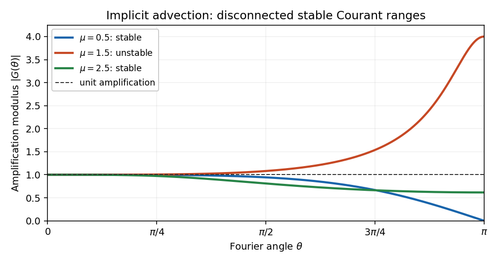
For a Fourier mode $U_j^n=G(\theta {)}^n{e}^{ij\theta }$, defineThe amplification factor is $G=N/L$. To derive its stability condition, use the coefficient abbreviations from the preceding solution and set $q=\cos \theta$. The squared moduli areHere $a+c={\mu }^2-\mu +1$, $a-c=2\mu -1$, and $4ac=K(\mu )$. Subtraction and factorization giveThus $|G|\le 1$ for every frequency exactly when $K(\mu )\ge 0$, provided the implicit denominator does not vanish. For the physically nonnegative Courant number, this givesFor a signed convention the full real range is $(-\infty ,-1]\cup [0,1]\cup [2,\infty )$.

There is no hidden denominator failure in these ranges. If $K>0$ and $L=0$, the identity forces $N=0$ and $\cos \theta =1$; but $N(0)=3$. If $K=0$, then $|L|=|N|$, and $N$ could vanish only when its two real coefficients have equal magnitudes. Their sum is three, so equality requires $\mu =1/2$, which is not a root of $K$. Hence $L$ is nonzero for every frequency in the allowed ranges. On the compact frequency interval its inverse is bounded for each fixed allowed $\mu$.

When $K<0$, choose a small nonzero frequency. The denominator remains close to three, while the boxed identity gives $|N|>|L|$. Its fixed-frequency numerical mode grows geometrically, proving instability in the usual fixed-Courant refinement limit. Conversely, for $K\ge 0$, the Plancherel theorem converts the mode bound into a discrete L2 norm contraction on the whole-line or periodic grid. The large-Courant branch is possible because the scheme is implicit; stability alone does not promise small error at a large step.

The Fourier sine basis of the unit square is $e_{j\ell }(x,y)=2\sin (j\pi x)\sin (\ell \pi y)$, $j,\ell \ge 1$, normalized in the L2 inner product. It satisfies the zero Dirichlet boundary conditions and $\Delta e_{j\ell }=-{\pi }^2(j^2+{\ell }^2)e_{j\ell }$. Expand the given initial datum as $u_0=\sum a_{j\ell }{e}_{j\ell }$, where $\sum |a_{j\ell }{|}^2=\Vert u_0{\Vert }_2^2$. The solution isFor $\kappa \le 2{\pi }^2$, every exponent is nonpositive. The series converges in $L^2$ for $t\ge 0$, tends to $u_0$ in $L^2$ as $t\downarrow 0$ by dominated convergence, and differentiates termwise for $t>0$ because the Gaussian high-frequency decay dominates every polynomial derivative factor. This constructs a classical positive-time solution and the appropriate mild solution at the possibly rough initial time.

Its norm and the difference of two such solutions satisfyExistence, uniqueness in the natural $L^2$ solution class, and continuous dependence follow. For uniqueness one can project any weak solution onto each sine mode, obtaining the same scalar linear equation and initial coefficient. Thus this is a Hadamard well-posed problem, with a contractive strongly continuous semigroup in the stated range.

To prove pointwise decay from merely $L^2$ data, use $|e_{j\ell }|\le 2$ and the Cauchy-Schwarz inequality:For $t\ge 1$, factor out $e^{2(\kappa -2{\pi }^2)t}$; the remaining sum is bounded by ${\sum }_{j,\ell \ge 1}{e}^{-2{\pi }^2(j^2+{\ell }^2-2)}<\infty$. ThereforeAt equality the first sine mode is stationary, so strict inequality is essential for decay of every datum. This is the Dirichlet heat-reaction threshold on the unit square. The equation is actually well posed on every fixed finite time interval for any fixed real $\kappa$; beyond the threshold it has a growing first mode and loses long-time contractivity. The restricted well-posedness assertion in the question is therefore sufficient rather than necessary.

Take $M$ interior points in each direction and spacing $h=1/(M+1)$. The one-dimensional Dirichlet discrete Laplacian has sine eigenvectors $v_i^{(j)}=\sin (j\pi ih)$, becauseThe five-point Dirichlet Laplacian as a Kronecker sum therefore has product eigenvectors $v_i^{(j)}{v}_r^{(\ell )}$. Adding the reaction term gives modal growth ratesThe semidiscrete matrix is real symmetric, so these modes are orthogonal in the mesh-weighted discrete L2 norm. Non-growth for all times is equivalent to every rate being nonpositive. The largest is ${\lambda }_{11}$, giving the five-point heat-reaction stability thresholdAt equality the first grid mode is neutral; above it that mode grows exponentially. This criterion concerns the spatially semidiscrete, continuous-time evolution. Any subsequent time integrator has an additional stability requirement.

The threshold expands as $2{\pi }^2-{\pi }^4{h}^2/6+O(h^4)$ and is below the continuum threshold for every finite mesh. Thus at the continuum neutral value the grid first mode has a small positive $O(h^2)$ rate. This is compatible with finite-time convergence, although it prevents an all-time contraction on that fixed mesh. In the weaker finite-time mesh-uniform sense, all fixed $\kappa$ have the bound $\Vert U(t){\Vert }_h\le e^{\kappa t}\Vert U(0){\Vert }_h$ because the discrete Laplacian is nonpositive. The boxed range is the natural non-growing stability range, matching the threshold comparison in the preceding part; finite-time stability versus power boundedness is a distinct question.

Work with real functions and $f\in L^2(0,1)$. To give the variational problem a definite domain, choose the homogeneous Dirichlet boundary conditions used in the next part. The natural form space is the zero-trace Sobolev space $H=H_0^1(0,1)$, with norm $\Vert v{\Vert }_H=\Vert v^{\prime }{\Vert }_2$. The Sobolev trace operator is well defined because one-dimensional $H^1$ functions have absolutely continuous representatives. For example $v(0)={\int }_0^{1}v(x)dx-{\int }_0^1(1-x)v^{\prime }(x)dx$, so its endpoint trace is bounded in the $H^1$ norm; the other endpoint has the analogous estimate. The zero-trace space is closed in the Hilbert space $H^1$, and the Poincaré inequality $\Vert v{\Vert }_2\le {\pi }^{-1}\Vert v^{\prime }{\Vert }_2$ makes the chosen derivative norm equivalent to its full norm. Thus $H$ is a Hilbert space.

Differentiability of $p,q$ implies continuity on the compact interval. Hence there are finite constants $p_{\max },q_{\max }$ and a positive $p_{\min }$ with $p_{\min }\le p\le p_{\max }$ and $0\le q\le q_{\max }$. Define the symmetric bilinear formThe Cauchy-Schwarz inequality and Poincaré inequality give all the estimates required by the Lax-Milgram theorem:That theorem states that a continuous coercive bilinear form on a Hilbert space and a bounded linear functional determine a unique weak solution. Completeness, continuity, coercivity and boundedness have now all been verified. Therefore there is a unique $u\in H$ with $a(u,v)=⟨f,v⟩$ for every $v\in H$.

The energy version of the given variational problem is $I(v)=a(v,v)-2⟨f,v⟩$. Its exact variation isBoundedness of $a$ makes the last term quadratic in $\Vert w{\Vert }_H$, so the Fréchet derivative is $DI(v)[w]=2a(v,w)-2⟨f,w⟩$. Its vanishing for every test function is preciselyTaking compactly supported smooth tests and integrating in the distributional sense shows that this is the Euler-Lagrange equation $-(p{u}^{\prime }{)}^{\prime }+qu=f$. Conversely that weak equation gives the displayed stationary condition. The stationary point is actually the unique global minimizer, becauseEquality occurs only when $v=u$. This proves the variational equivalence, including existence and uniqueness rather than only a formal derivative calculation.

For precision about the literal L2 inner product $⟨Lv,v⟩$, use the flux-domain realization of a one-dimensional elliptic operatorFor such $v$, weak integration by parts and its zero endpoint values give $⟨Lv,v⟩=a(v,v)$. On the larger form space $H$, the same energy is interpreted by the weak operator pairing. The minimizer belongs to $D(L)$ automatically: its weak equation gives $(p{u}^{\prime }{)}^{\prime }=qu-f\in L^2$, while $p{u}^{\prime }\in L^2$. Thus its equation also holds as an equality of $L^2$ functions. This domain does not assume bounded $p^{\prime }$, which mere differentiability would not supply. If $p\in C^1$ one may equivalently use $D(L)=H^2\cap H_0^1$, but that stronger coefficient assumption is not needed for the proof here.

Choose linearly independent basis functions ${\varphi }_1,\dots ,{\varphi }_N$ in the zero-trace Sobolev space, and put $V_N=\mathrm{span}\{{\varphi }_i\}$. A concrete conforming Galerkin method uses continuous piecewise-linear hat functions on an interval mesh, with zero endpoint values. Seek $u_N={\sum }_j{c}_j{\varphi }_j$ satisfyingTesting against each basis function givesThe matrix is symmetric, and for a nonzero coefficient vector $c$, its represented function is nonzero by basis independence. The coercivity estimate gives $c^{T}Kc=a(u_N,u_N)>0$. Thus $K$ is a positive-definite matrix, the finite-dimensional problem has a unique solution, and it minimizes the same energy over $V_N$. This is Ritz-Galerkin equivalence for a symmetric coercive form.

Subtracting the continuous and discrete equations proves Galerkin orthogonality: $a(u-u_N,v_N)=0$ for all $v_N\in V_N$. Let $\Vert v{\Vert }_a=\sqrt{a(v,v)}$. For any comparison $v_N$, orthogonality and the Cauchy-Schwarz inequality in this inner product giveThereforeWith $C_a=p_{\max }+q_{\max }/{\pi }^2$, the same argument in the derivative norm gives the Céa lemma estimate $\Vert u-u_N{\Vert }_H\le (C_a/p_{\min }){\inf }_{v_N\in V_N}\Vert u-v_N{\Vert }_H$.

Convergence now follows from approximation, not from a bare assertion that the residual is small. The defining density of smooth compactly supported functions in $H_0^1$ lets one approximate $u$ by such a smooth function. Its piecewise-linear interpolant has zero endpoints and derivative error tending to zero as the largest mesh interval tends to zero. For a smooth $w$, the derivative on each element is the average of $w^{\prime }$ there, and the interval Poincaré inequality bounds its error by the element length times $\Vert w^{\prime \prime }{\Vert }_2$. Density and the boxed best-approximation estimate consequently give $u_N\to u$ in $H_0^1$, and hence in $L^2$, without assuming a bounded derivative of $p$. If the stronger regularity $u\in H^2$ is available, the same interpolation estimate gives first-order convergence in the derivative norm.

A collocation Runge-Kutta method approximates an ordinary differential equation by a polynomial whose derivative agrees with the vector field at selected times. Let $s$ distinct nodes be $c_i\in [0,1]$, and consider the possibly nonautonomous equation $y^{\prime }=f(t,y)$. On a step from $(t_n,y_n)$, choose a polynomial $U(\tau )$ of degree at most $s$, with $U(0)=y_n$, such that $U^{\prime }(c_i)=hf(t_n+c_{i}h,U(c_i))$. Here $\tau =(t-t_n)/h$ is scaled time; the numerical endpoint is $y_{n+1}=U(1)$.

Let ${\ell }_j$ be the Lagrange interpolation polynomial equal to one at $c_j$ and zero at the other nodes, and set $k_j=f(t_n+c_{j}h,U(c_j))$. Interpolation of the polynomial derivative givesEvaluating at the nodes and endpoint derives the Runge-Kutta method coefficients:Thus collocation is a specific family of generally implicit RK methods, not a separate update mechanism. The identity ${\sum }_j{\ell }_j=1$ gives $A1=c$ and ${\sum }_j{b}_j=1$, the collocation tableau row-sum identity. For sufficiently small $h$, a vector field with Lipschitz constant $L$ gives a contraction of the stage map when $hL{\max }_i{\sum }_j|a_{ij}|<1$, on a suitable bounded neighborhood. The Banach fixed-point theorem then gives a unique nearby stage solution. Equivalently smooth stage equations have identity derivative in the stage variables at $h=0$, so the inverse function theorem gives a smooth nearby branch. Arbitrarily large-step solvability is a separate issue for an implicit Runge-Kutta method.

Order analysis has two levels: polynomial accuracy at stages and extra accuracy at the endpoint. Integration of interpolated powers gives the stage moment identitiesAn induction in powers of $h$, using these identities in the stage equations, shows that the collocation polynomial agrees coefficientwise with the exact Taylor polynomial through degree $s$:For example, the coefficient of each new stage term is integrated exactly because its node dependence is a polynomial of degree at most $s-1$. This proves stage order $s$ and bounded actual-time derivatives of the collocation polynomial up to degree $s$. Assuming the vector field is sufficiently smooth on a fixed compact solution neighborhood, its composition with this polynomial has uniformly bounded derivatives of all finite orders needed below.

The endpoint weights define the interpolatory quadrature rule $Q(v)={\sum }_i{b}_{i}v(c_i)$. Suppose it is exact through degree $q-1$, but not through degree $q$. Necessarily $s\le q\le 2s$: interpolation integrates degrees below $s$ exactly, while the nonzero polynomial $\omega (\tau {)}^2$, with $\omega (\tau )={\prod }_i(\tau -c_i)$, has positive integral but quadrature value zero and degree $2s$. Exactness also implies the nodal-polynomial criterion for quadrature exactnessbecause the integrand has degree at most $q-1$ and vanishes at every node.

Here is the endpoint-error argument underlying the collocation order theorem. Let $v(t)=U((t-t_n)/h)$ and $\delta (t)=v^{\prime }(t)-f(t,v(t))$ be its residual. It vanishes at the collocation times, and if $F_h(\tau )=f(t_n+h\tau ,U(\tau ))$, then $\delta ={\mathcal{I}}_s{F}_h-F_h$, where ${\mathcal{I}}_s$ is interpolation at the nodes. Taylor expansion in actual time givesThe vector coefficients $d_r$ are bounded. Each bracket has the factor $\omega (\tau )$, with quotient degree $r-s$. In particular the residual is $O(h^s)$ throughout the step.

Write $\varphi (t_{\ast },t,z)$ for the exact flow from time $t$ and state $z$ to $t_{\ast }=t_n+h$. Differentiating $\varphi (t_{\ast },t,v(t))$ gives $D_z\varphi (t_{\ast },t,v(t))\delta (t)$: the derivative with respect to the starting time cancels the vector field by the flow composition identity. Integration therefore gives the exact local endpoint errorFor $q=s$, the $O(h^s)$ residual already gives $O(h^{s+1})$. For $q>s$, Taylor-expand the smooth matrix weight as $\Psi (t_n+h\tau )={\sum }_{\ell =0}^{q-s-1}{h}^{\ell }{\Psi }_{\ell }{\tau }^{\ell }+O(h^{q-s})$. Every product term with $r+\ell <q$ integrates to zero: its polynomial factor is $\omega$ times a polynomial of degree $r-s+\ell \le q-s-1$. All remaining terms are $O(h^q)$ before the time integration, including both remainders. HenceThis is collocation endpoint superconvergence by quadrature orthogonality. For the global assertion, the stage contraction estimate gives a one-step Lipschitz bound $1+Ch$ on a fixed solution neighborhood. Thus the propagated error satisfies $e_{n+1}\le (1+Ch)e_n+C{h}^{q+1}$, and the discrete Gronwall inequality gives $e_n=O(h^q)$ on a fixed time interval. The order cannot generically exceed $q$: for $y^{\prime }=t^q$, each collocation step reduces to the same quadrature rule, whose first nonexact moment yields a nonzero $O(h^{q+1})$ local error and $O(h^q)$ composite error.

The usual node families illustrate the result. Gauss collocation methods use interior Gaussian nodes and have $q=2s$, the maximum possible order. Right-endpoint Radau nodes give the Radau IIA method of order $2s-1$. Including both endpoints with Lobatto quadrature gives the Lobatto IIIA method of order $2s-2$ for $s\ge 2$. One-stage Gaussian collocation is the second-order implicit midpoint rule, while collocation at the right endpoint is the first-order Backward Euler method. The two-stage Gaussian nodes $1/2\pm \sqrt{3}/6$ give $b=(1/2,1/2)$ anda fourth-order method. Node placement, rather than just stage count, controls the superconvergent endpoint order.

There is also a structural link with Question 2. For Gaussian nodes, let $L_i(\tau )={\int }_0^{\tau }{\ell }_i(v)dv$. The derivative of $L_i{L}_j$ has degree at most $2s-1$, so Gaussian quadrature is exact on it. The integral is $b_i{b}_j$, while evaluating at the nodes gives $b_i{a}_{ij}+b_j{a}_{ji}$. Thus Gaussian collocation satisfies $M=0$ and has Runge-Kutta conservation of quadratic invariants. For the scalar test equation, any RK method has stability function $R(z)=1+z{b}^T(I-zA{)}^{-1}1$. For implicit midpoint this is $(1+z/2)/(1-z/2)$; the identity $|1-z/2{|}^2-|1+z/2{|}^2=-2\mathrm{Re}z$ proves A-stability. High order, stage solvability, invariant preservation and damping are distinct design considerations, so no stability conclusion should be inferred from collocation order alone.

Fourier stability analysis exploits translation invariance of a linear constant-coefficient finite difference method. On an infinite uniform grid of spacing $h$, a spatial shift acts on $e^{ij\theta }$ by multiplication by $e^{i\theta }$. Hence a scalar two-level scheme with new- and old-time symbols $L(\theta ),N(\theta )$ propagates each Fourier mode by $G(\theta )=N(\theta )/L(\theta )$, provided the new-time operator is invertible. An explicit stencil $U_j^{n+1}={\sum }_{\ell }{a}_{\ell }{U}_{j+\ell }^n$ simply has $G(\theta )={\sum }_{\ell }{a}_{\ell }{e}^{i\ell \theta }$. This converts a spatial evolution into scalar algebra at each frequency.

The Plancherel theorem gives the full norm estimate, rather than just a heuristic about waves. For the discrete Fourier transform $\hat{U}(\theta )={\sum }_j{U}_j{e}^{-ij\theta }$, interpreted in the $L^2$ sense if necessary,Thus a scalar mode bound gives an exact discrete L2 norm bound. Stability on a fixed physical interval requires constants independent of the refining spatial and time meshes:The contraction condition $|G|\le 1$ is sufficient and customary for equations whose exact solutions do not grow. More generally $|G|\le 1+Ck$ suffices, since $(1+Ck{)}^n\le e^{CT}$. At a fixed Courant number, when $G$ is independent of $k$, a mode with modulus strictly greater than one violates the estimate as $n\sim T/k\to \infty$. One must keep this scaling: physical growth such as $e^{\kappa t}$ does not by itself mean finite-time numerical instability. This is finite-time stability versus power boundedness.

For systems, the symbol is an amplification matrix. The requirement is a uniform bound on all its powers, not merely its eigenvalues. A unit-modulus Jordan block $\left(\begin{array}{cc}1& 1\\ 0& 1\end{array}\right)$ has powers $\left(\begin{array}{cc}1& n\\ 0& 1\end{array}\right)$ and is unstable under refinement. A uniformly conditioned eigenbasis or an energy estimate can justify a modal conclusion; eigenvalues alone cannot control a general nonnormal matrix. Multilevel schemes likewise produce an amplification polynomial of a multilevel finite difference scheme, with a uniform root condition and control of starting errors. Repeated unit-modulus roots can give polynomial growth, and roots approaching each other require attention to mesh-uniform constants.

Several elementary examples show how the calculation works. For $u_t+c{u}_x=0$ with $c>0$, forward Euler with centered spatial differences gives $G=1-i\mu \sin \theta$, where $\mu =ck/h$. Since $|G{|}^2=1+{\mu }^2{\sin }^2\theta$, it is unstable at every fixed nonzero Courant number. The upwind finite difference scheme instead gives $G=1-\mu +\mu e^{-i\theta }$ andso its exact contraction range is $0\le \mu \le 1$. The Lax-Wendroff advection scheme has $G=1-i\mu \sin \theta +{\mu }^2(\cos \theta -1)$; expansion gives $|G{|}^2=1-4{\mu }^2(1-{\mu }^2){\sin }^4(\theta /2)$, hence $|\mu |\le 1$. The Courant–Friedrichs–Lewy condition relates these restrictions to the numerical domain of dependence, but is a necessary geometric check rather than a complete stability proof. Implicit schemes can have a global spatial dependence and different Courant ranges, as Question 3 illustrates.

For the heat equation $u_t=\nu u_{xx}$, put $r=\nu k/h^2$. Central spatial differences with forward Euler give $G=1-4r{\sin }^2(\theta /2)$, so $0\le r\le 1/2$. With backward Euler the factor is $[1+4r{\sin }^2(\theta /2){]}^{-1}$, a contraction for every $r\ge 0$. For the Crank-Nicolson diffusion scheme it is $[1-2r{\sin }^2(\theta /2)]/[1+2r{\sin }^2(\theta /2)]$, again a contraction for all $r\ge 0$. At large $r$, however, high-frequency factors approach minus one rather than zero: unconditional stability does not imply strong damping or accurate resolution of every mode.

The connection with convergence is the Lax equivalence theorem for a consistent approximation to a well-posed linear evolution problem. Its forward implication follows directly from the error recursion. If $e^{n+1}=G_h{e}^n+k{\tau }^n$ and $\Vert G_h^j\Vert \le C_T$ for $jk\le T$, thenA convergent initialization and a vanishing normalized local truncation error therefore give convergence. Smooth-data consistency can be extended by density when the approximation and initialization are uniformly bounded. For rough $L^2$ data, cell averages or another L2-compatible initialization of grid data are preferable to undefined point samples. A high formal order does not rescue an unstable amplification operator.

Boundary conditions determine whether Fourier diagonalization is exact. On a periodic grid the update is a circulant matrix, and the finite discrete Fourier transform diagonalizes it at the frequencies $2\pi \ell /N$. Here an interior symbol controls the entire scheme, including the wrapping boundary. On the whole line, the continuous frequency transform serves the same purpose and there is no boundary closure to check.

For a finite interval with homogeneous Dirichlet boundary conditions, centered diffusion is a symmetric tridiagonal problem diagonalized by discrete sine modes. One tests the same diffusion symbol at the admitted sine frequencies, not at arbitrary periodic modes. For homogeneous Neumann boundary conditions, a suitable reflected closure uses discrete cosine modes; the constant mode is present and is neutral for pure diffusion. With the standard reflected endpoint stencil, the natural norm uses half endpoint weights, in which the matrix is self-adjoint. Consequently stable diffusion need not make every solution tend to zero under Neumann conditions. These special orthogonal bases supply an exact substitute for Fourier modes when the operator and closure have the required symmetry.

For transport, prescribe only the incoming physical boundary data. With $u_t+c{u}_x=0$, $c>0$, the inflow is the left endpoint; for $u_t=u_x$ it is the right endpoint. Imposing unrelated data at both ends generally overdetermines the first-order PDE. Outflow rows or ghost points must be chosen compatibly with the interior method. A general boundary closure of a difference scheme destroys the circulant structure, so whole-line von Neumann stability analysis is necessary in many settings but not sufficient for the full initial-boundary problem. A defective boundary row that doubles one boundary unknown each step can create growth even beside a stable interior stencil.

A more refined boundary calculation seeks half-line modes $U_j^n=w^n{\zeta }^j$ with $|\zeta |<1$; these are localized near the boundary. Insert them into both the interior recurrence and boundary equations. A compatible mode with $|w|>1$ proves boundary instability. Absence of one isolated growing mode is not the whole theorem: weakly controlled limiting modes can still destroy a uniform estimate. The Uniform Kreiss--Lopatinskii condition requires a uniformly bounded inverse boundary system on the incoming/decaying mode space. Direct energy estimates are often a clearer alternative to solving that transformed boundary problem.

For example, suppose a first-derivative matrix obeys the discrete summation by parts identity $HD+D^{T}H=e_N{e}_N^T-e_0{e}_0^T$, with positive norm matrix $H$. The semidiscrete advection equation $U_t=-cDU$ then givesWith homogeneous inflow $U_0=0$ and $c>0$, only a nonpositive outflow term remains; prescribed inflow contributes a controlled forcing term. This is the inflow advection energy estimate from summation by parts, and it tests the boundary as part of the operator. For a dissipative semidiscrete matrix $A$, backward Euler also preserves the estimate, because its update givesThis distinguishes spatial energy stability from stability of an arbitrary chosen time integrator.

Finally, nonhomogeneous boundaries can be homogenized by subtracting a suitable lifting, leaving a forced equation whose solution needs a bound in terms of both initial and boundary data. Variable coefficients and nonuniform grids remove translation invariance, so freezing coefficients gives only local diagnostic information. A full energy method, a mesh-uniform operator estimate, or a dedicated boundary-symbol analysis is then needed. Fourier symbols give complete stability tests when an orthogonal mode decomposition diagonalizes the full operator; otherwise the boundaries, matrix powers and norm estimates must be checked as well.