Assume the decreasing functions are continuously differentiable so their local gains are defined. In the positive quadrant, the nullclines are and , both decreasing. The phase plane arrows point right when and left when ; they point up when and down when . Both axes point into the quadrant. Since are bounded, sufficiently large or decreases, giving a bounded forward-invariant rectangle containing all equilibria and eventually containing each trajectory. Thus mutual repression can have one attracting intersection or several intersections separating different basins of attraction.
An equilibrium obeys , . Its Jacobian matrix and eigenvalues areThe product is nonnegative. Hence an intersection is a stable equilibrium with two negative real eigenvalues when , a saddle equilibrium when , and nonhyperbolic when . This is the mutual repression stability criterion. To see why an intervening saddle normally accompanies multistability, eliminate and set . Bounded positivity gives and for large , whileTwo downward, stable crossings require an upward crossing between them. For simple roots that middle crossing has and is a saddle equilibrium. Its stable manifold separates the attracting states. Thus robust multistability requires the loop gain to exceed one at an intervening equilibrium, with the stable equilibria themselves having gain below one. A tangency at gain one is the threshold where equilibria can merge; degenerate crossings require higher-order analysis. A gain exceeding one somewhere is necessary for multiple intersections, but by itself does not prove that a particular pair of nullclines has multiple stable intersections.
Define the logarithmic repression sensitivitiesBoth are negative. At equilibrium and , so their product is exactly . The condition can therefore be expressed asEquivalently, the product of the magnitudes of the two negative logarithmic gains must exceed one at that saddle equilibrium. The divergence of the vector field is identically , so the Bendixson-Dulac criterion excludes periodic orbits in the positive quadrant. The relevant stable long-time states in this bounded phase plane are thus equilibria, rather than attracting limit cycles. The following sketches illustrate the single-attractor and two-attractor possibilities; the saddle in the second panel lies on the diagonal, with its stable diagonal separating the two basins.
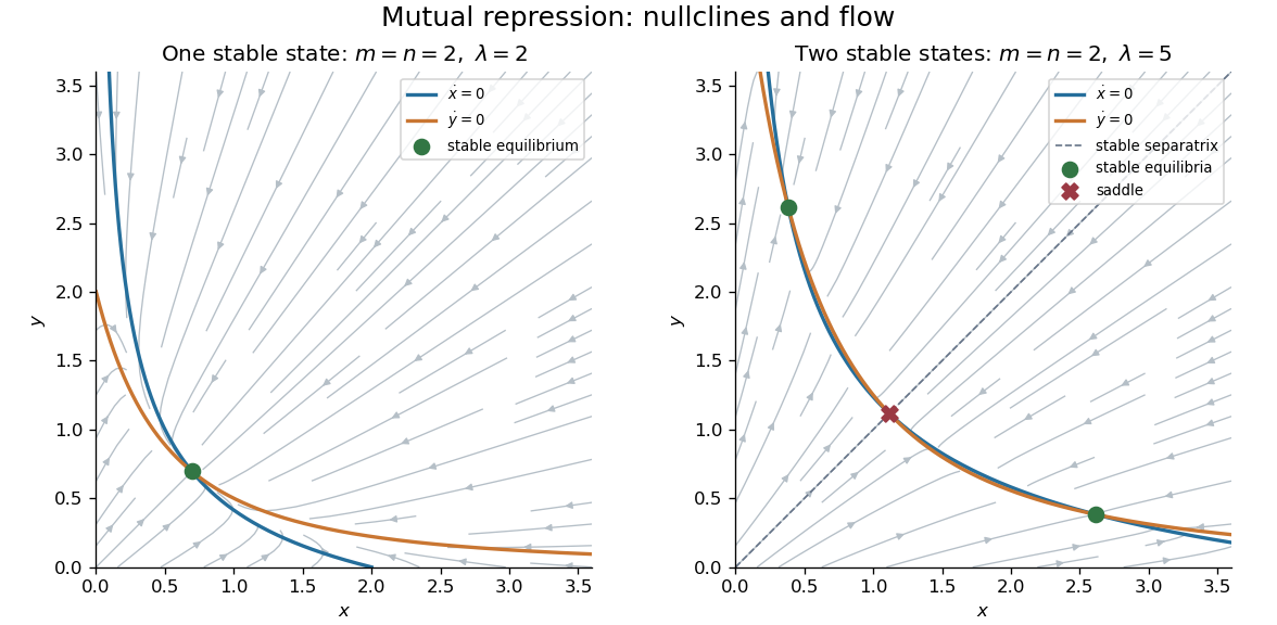
Mutual repression phase planes: one stable equilibrium and two stable equilibria separated by a saddle equilibrium
. Details. 
For this equal-strength power-law mutual repression, the logarithmic gains and their product at equilibrium areThe mutual repression stability criterion immediately excludes multistability if , since at every finite positive equilibrium. The common prefactor gives a stronger exclusion: if either exponent is at most one, multistability is impossible for every , including some cases with .
To prove the additional cases, suppose . At equilibrium the two expressions for implyPut and . Because , the left side is at least , so . It follows thatThe maximum in the second inequality occurs at . Its strict bound follows from , , and . Interchanging the components proves the case ; the case with both exponents at most one was already covered by . Every root of therefore has . Since begins positive and ends negative, there is exactly one root: two downward crossings would require another crossing with nonnegative derivative between them. The unique equilibrium is stable.
For completeness, neither exponent can be relaxed above one in this exclusion. If and , take sufficiently large. On , , so maps that interval into itself. It has a fixed point withIt is a stable equilibrium. By exchanging the components, there is a second stable fixed point with and . These two regions are disjoint for large , proving bistability for some production strength. Hence the full answer isFor example, has but still a unique stable equilibrium for all . Thus the product-only necessary condition for strong feedback is not sufficient when both production prefactors are constrained to be equal.
Let . The Markov jump-process generator applied to gives the exact moment equation . With the prescribed moment closure, , stationarity givesThe production flux counts molecules, not reaction events: it is , while the removal flux is . The reaction-rate elasticity of removal relative to constant production isThe mean molecular lifetime is population divided by its stationary molecular removal flux. ThereforeThe noise-relevant average chemical event size is the molecular-flux-weighted reaction event size. For the stoichiometric vectors and it isThis weights each absolute jump by the molecular turnover it contributes. Equivalently, the balanced production and removal fluxes give equal weight to their sizes and , yielding . An event-count-weighted average would be , since three quarters of firing events are deaths at stationarity; that different average does not determine the diffusion term in the linear noise approximation.
The normalized stationary fluctuation-dissipation relation for a reaction network isHere is the negative drift Jacobian matrix expressed in normalized population coordinates, and is the normalized noise matrix. More explicitly, with , drift Jacobian , stoichiometric vectors , and stationary reaction propensity functions , these matrices are and , where . The linear noise approximation gives a covariance evolution ; stationarity is the displayed Continuous Lyapunov equation.
In one dimension, the normalized restoring coefficient is . Squared chemical jumps determine the noise:The factor nine from a birth burst is essential; its three molecules arise in one correlated reaction event. The scalar Continuous Lyapunov equation is , givingEquivalently, the normalized variance is . The Fano factor is approximately four. This calculation uses the prescribed mean closure and the linear noise approximation, so its small-relative-fluctuation regime is ; it is not an exact assertion for arbitrarily small molecular copy numbers.
For the Gillespie algorithm, start from and an integer molecular copy number . At each step use the current state, without the mean approximation in parts (a)–(b). The reaction propensity functions are and , and their sum is . Draw two independent uniform random variables on and setThe waiting time has an exponential distribution with rate . Keep the sample path constant on , advance , and choose the reaction byRecord the post-jump state, recompute both reaction propensity functions, and repeat with fresh independent uniforms. At the death propensity is zero, so only a birth is selected and the trajectory remains nonnegative. For a prescribed terminal time , if the next event would occur after , keep the current state to and stop. This produces exact piecewise constant sample paths of the specified continuous-time Markov chain.
Let . Applying the Markov jump-process generator to either coordinate gives the exact moment equationsIn each equation the joint reaction removes one molecule, at reaction propensity function . Because the two reactants are different chemical species, the propensity uses their product; no same-species factorial correction is needed. The exact identity shows explicitly where the equations fail to close. Neglecting this covariance relative to the product of means is the small-fluctuation moment closure. It gives the mean-field joint removal of two chemical species:The difference equation actually holds exactly as well as after closure, because both the constant production and the joint removal terms cancel. The nonlinear moment closure will be used for the subsequent phase plane and stationary linear noise approximation calculations, as requested.
Use the approximate reaction-rate equations from part (a), with axes and . In every case the positive quadrant is forward invariant, since the drift on either zero-concentration axis points inward. The nullclines specify the arrow signs: right if , left if the inequality is reversed; up if , down otherwise.
For and , the nullclines are the vertical line and the horizontal line . The two components relax independently:Every nonstationary trajectory is a straight ray towards the unique stable equilibrium , whose Jacobian matrix is .
For and , both derivatives equal , so the two nullclines coincide onEvery point of this hyperbola is an equilibrium. The difference is conserved, and trajectories therefore run along straight lines of slope one. Below the hyperbola they point up and right; above it they point down and left. Each such line converges to its own intersection with the hyperbola,At this point the Jacobian matrix is , with eigenvalues and . Thus the equilibrium curve attracts transversely but has no restoring drift along its tangent. Its points are not individually asymptotically stable, because arbitrarily close initial states on different constant-difference lines converge to different equilibria.
For and , the nullclines are the decreasing curves and , reflected in the diagonal. At an intersection, subtracting the two stationary equations gives . Hence there is exactly one intersection, whereThe Jacobian matrix at this point isIts symmetric eigenvector has eigenvalue , and the antisymmetric eigenvector has eigenvalue . Both are negative, so the symmetric equilibrium is a stable node. All trajectories are bounded because each component above decreases. The divergence excludes periodic orbits by the Bendixson-Dulac criterion, and the unique interior equilibrium attracts the positive-quadrant trajectories. As becomes small, the drift restoring the difference becomes slow, so paths first approach the near-hyperbolic nullclines and then drift towards the symmetric intersection. These sketches show the three cases printed in the PDF; the middle case is , not the different cases introduced by the converted TeX.
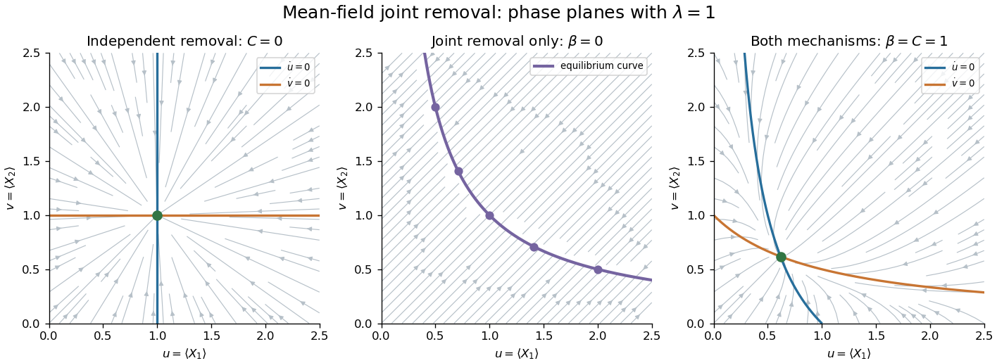
Mean-field phase planes with independent removal, exclusive joint removal, and both removal mechanisms
. Details. 
For , symmetry of the unique stationary mean-field state gives and the balance . The fraction of the molecular removal flux using the joint reaction and the mean molecular lifetime are consequentlyIn particular , , and .
The total loss flux of species one is , whereas its production flux is constant. The reaction-rate elasticities are therefore and at the symmetric state. Species two gives , . All chemical jumps in either component have unit absolute size, so their molecular-flux-weighted reaction event sizes satisfy . With , this provesThe same matrix follows from with and the drift Jacobian matrix in part (b); its positive eigenvalues are the restoring rates.
For the chemical diffusion matrix, each component receives noise from one unit birth, its own unit death, and the joint unit loss. The unnormalized diagonal noise intensity isOnly the joint reaction changes both components in one event. Its stoichiometric vector is , so . The positive sign reflects simultaneous decreases, rather than independent death events. Divide by the product of the means to normalize:Thus the chemical diffusion matrix in the normalized stationary fluctuation-dissipation relation for a reaction network isThe unequal roles of and matter: describes restoration of perturbations, while records the covariance of the immediate stochastic reaction increments.
By symmetry the normalized covariance matrix has the form . Substituting the matrices from part (c) into the normalized stationary fluctuation-dissipation relation for a reaction network, , givesHence and . Solving these two equations gives the linear noise of two species with joint removal:For the normalized variance is and the covariance is zero, as expected for independent immigration–death processes. For , exceeds this independent value and . The correlation coefficient isThis negative stationary correlation is compatible with positive instantaneous joint-removal noise: the slow difference mode amplifies fluctuations of opposite signs in the two populations.
The symmetric and antisymmetric eigenvectors diagonalize all three matrices. Their normalized covariance eigenvalues areThe corresponding restoring rates are and . Thus the sum mode retains finite fluctuations, with , whereas the difference mode becomes arbitrarily noisy. In particular, at a fixed nonzero mean, or along at fixed so ,The Fano factor of either population is , which diverges as regardless of how the mean is varied. Unnormalized variances are and covariance , so their absolute magnitudes also depend on the parameter path through .
The phase plane in part (b) explains the singularity. At , the mean-field system has a whole hyperbola of equilibria, rather than an isolated restoring state. A perturbation in the species difference selects another point on that curve. In the actual stochastic reaction network, joint complex formation still leaves unchanged, but the two constant-rate births change it by and , each at rate . Therefore exclusive joint removal has a diffusing difference mode:Its continuous-time symmetric simple random walk on the integers has no normalizable stationary distribution, so there is no finite stationary covariance at . The divergence as signals both the loss of difference-mode restoration and eventual failure of the small-fluctuation moment closure; near the limit, the computed normalized variances need not remain small even when the individual mean populations are large.
Articles by others on the same topic
There are currently no matching articles.