Past exam of the mathematics course of the University of Cambridge / 2008 / iii / Paper 74 (Stellar and Planetary Magnetic Fields)

Let the basic temperature be $\overline{T}=T_{\ast }-\beta z$ with $\beta >0$, the density be ${\rho }_0$, gravitational acceleration be $-g\hat{\mathbf{z}}$, and thermal expansion coefficient be $a_T$. Denote kinematic viscosity, thermal diffusivity and magnetic diffusivity by $\nu ,\kappa ,\eta$. Write the dimensional magnetic perturbation as ${\mathbf{b}}_d$, the temperature perturbation as ${\theta }_d$, and use constant permeability ${\mu }_0$. Linearizing the Boussinesq equations and the resistive induction equation about the static state givesThe Lorentz force identity is $(\nabla \times {\mathbf{b}}_d)\times B_0\mathbf{c}=B_0(\mathbf{c}\cdot \nabla ){\mathbf{b}}_d-\nabla (B_0\mathbf{c}\cdot {\mathbf{b}}_d)$. Its gradient term is absorbed into $P_d$, the perturbation magnetohydrodynamic total pressure. The temperature source follows from ${\mathbf{u}}_d\cdot \nabla \overline{T}=-\beta u_{d,z}$.

Choose any reference length $d$, since no vertical boundaries are prescribed. Scale length by $d$, time by $d^2/\kappa$, velocity by $\kappa /d$, temperature perturbation by $\beta d$, magnetic perturbation by $B_0$, and total pressure by ${\rho }_0\nu \kappa /d^2$. The dimensionless parameters areThey are the Prandtl number, magnetic-to-thermal diffusivity ratio, Rayleigh number, and Chandrasekhar number, respectively. Division by the chosen scales givesIn particular $Q\zeta =B_0^2{d}^2/({\mu }_0{\rho }_0\nu \kappa )$, so the diffusivity convention agrees with the momentum coefficient.

For a plane wave put $\mathbf{l}=(k,0,m)$, $q=|\mathbf{l}{|}^2=k^2+m^2$, and $d_{\parallel }=\mathbf{c}\cdot \mathbf{l}=k\sin \alpha +m\cos \alpha$. The induction and temperature equations imply $\hat{\mathbf{b}}=i{d}_{\parallel }\hat{\mathbf{u}}/(s+\zeta q)$ and $\hat{\theta }=\hat{w}/(s+q)$. The projection $P=I-\mathbf{l}{\mathbf{l}}^{\mathsf{T}}/q$ removes pressure. Because $(P\hat{\mathbf{z}}{)}_z=k^2/q$, its vertical momentum equation isThus the oblique-field plane-wave magnetoconvection dispersion relation isIf out-of-plane velocity is also allowed, its decoupled magnetic branch satisfies $(s/\sigma +q)(s+\zeta q)+Q\zeta d_{\parallel }^2=0$; it has no buoyant driving. At stationary marginality, for $k\ne 0$,These are stationary thresholds; an oscillatory marginal mode, if present for particular diffusivity ratios, is a different onset calculation.

For $m=1$, write $R_{mathrmstat}=F(k)+QG(k)$, where $F=(1+k^2{)}^3/k^2$ and $G=(1+k^2)(\cos \alpha +k\sin \alpha {)}^2/k^2$. Direct differentiation gives $F^{\prime }(k)=-2k^{-3}+6k+4k^3$, so its two minima are $\pm 1/\sqrt{2}$, with $F=27/4$ and $F^{\prime \prime }=36$. For $Q>0$ the negative sign has the smaller magnetic penalty: at every positive $k$, $G(-k)<G(k)$ because both sine and cosine of the inclination are positive. The wavenumber selection in oblique-field magnetoconvection therefore starts from $a=-1/\sqrt{2}$. Expanding $F^{\prime }(k_c)+Q{G}^{\prime }(k_c)=0$ gives $k_c=a+C_{1}Q+O(Q^2)$, where $C_1=-G^{\prime }(a)/F^{\prime \prime }(a)$. Taylor expansion of the value then givesThis proves the small-field forms, including the order of the correction.

For large $Q$, $G$ is nonnegative and vanishes only at $b=-\cot \alpha$. The candidate $k=b$ has finite threshold $F(b)$, so a global minimizer must satisfy $QG(k_c)\le F(b)$ and hence tend to $b$. Here $G^{\prime \prime }(b)=2(1+b^2){\sin }^2\alpha /b^2>0$. Expanding the stationarity condition at $b$ yieldsThe value expansion isThe leading coefficient follows from $1+{\cot }^2\alpha ={\csc }^2\alpha$. The expansion holds at fixed $0<\alpha <\pi /2$.

Finally choose $\cot \alpha =1/\sqrt{2}$. Then the nonmagnetic minimizing wavevector also has $d_{\parallel }=0$, and its magnetic penalty vanishes. Since $F(k)\ge 27/4$ and $QG(k)\ge 0$, this is the global minimum for every nonnegative field strength:This field-independent stationary threshold in oblique magnetoconvection has a simple physical explanation: the disturbance is constant along the imposed field, so it does not bend field lines.

The ansatz gives $B_r=A_{\varphi }/r$, $B_{\varphi }=-A_r$, and $B_z=B$. Initially $A=B_{0}r\sin \varphi$ and $B=0$, since $B_r=B_0\cos \varphi$ and $B_{\varphi }=-B_0\sin \varphi$ are a uniform Cartesian field. In ideal magnetohydrodynamics, the transverse flux function is advected, while the axial field is stretched by the axial velocity gradient. More explicitly, the transverse induction equations are equivalent to $({\partial }_t+f{\partial }_{\varphi })A=0$; the axial component of ${\partial }_t\mathbf{B}+\mathbf{u}\cdot \nabla \mathbf{B}=\mathbf{B}\cdot \nabla \mathbf{u}$ is $({\partial }_t+f{\partial }_{\varphi })B=B_r{g}^{\prime }$. Substituting the azimuthal mode therefore givesThe initial coefficients are $\hat{A}(r,0)=B_{0}r$ and $\hat{B}(r,0)=0$. Multiplication by $e^{ift}$ integrates both equations, giving $\hat{A}=B_{0}r{e}^{-ift}$ and $\hat{B}=i{B}_{0}t{g}^{\prime }{e}^{-ift}$. Thus the ideal magnetic response to a cylindrical cyclonic event at its end isWith ideal induction these fields remain frozen after the flow is switched off. The EMF calculated below is the active-flow value at $T^{-}$; at $T^{+}$ the velocity itself is zero.

In cylindrical components, $\mathbf{u}\times \mathbf{B}=(rfB+g{A}_r)\hat{\mathbf{r}}+(g{A}_{\varphi }/r)\hat{\mathbf{\varphi }}-f{A}_{\varphi }\hat{\mathbf{z}}$. Put $\psi =\varphi -fT$. Since $A_r=B_0(\sin \psi -rT{f}^{\prime }\cos \psi )$, its Cartesian $x$-component reduces toUse ${\int }_0^{2\pi }\cos \varphi \cos (\varphi -fT)d\varphi =\pi \cos (fT)$ and the area element $rdrd\varphi$. The integrated electromotive response of a finite cyclonic event isWhen the boundary term vanishes, the last two terms combine as $-g{\partial }_r[r^2\sin (fT)]$, giving the useful equivalent integralFor the compactly supported profile, $f{g}^{\prime }-g{f}^{\prime }=0$ on $0<r<a$. Substitution of $v=a^2-r^2$ into the first integral givesAt zero the continuous limiting value is zero, and $\mathcal{E}(T)=-\pi B_0{a}^{6}T/3+O(T^3)$. For $B_0>0$ it begins negative; the nonzero zeros satisfy $\tan (a^{2}T)=a^{2}T$, the first at $a^{2}T\simeq 4.4934$. It then alternates sign, with an asymptotic $1/T$ envelope. The requested sketch uses $x=a^{2}T$ and scales the EMF by $\pi B_0{a}^4$:

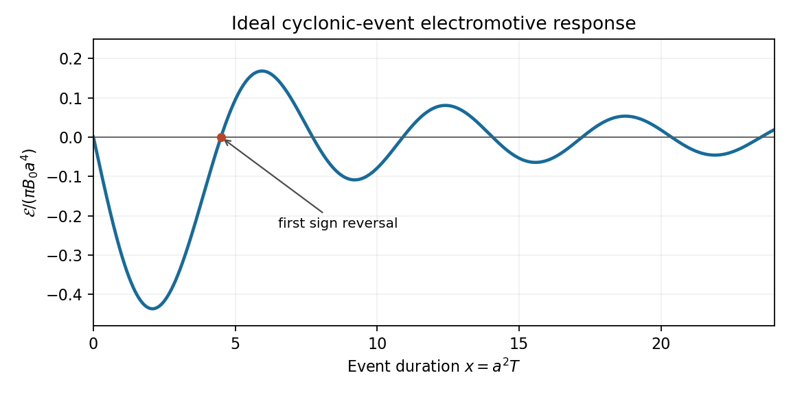
This sign alternation is possible even though the flow has fixed-sign kinetic helicity. Indeed, its vorticity components are $(0,-g^{\prime },2f+r{f}^{\prime })$, so $\mathbf{u}\cdot \mathbf{\omega }=2fg+r(g{f}^{\prime }-f{g}^{\prime })$, which reduces to $2f^2\ge 0$ for this profile. The finite-duration response retains winding and phase information; it cannot be assigned a universal sign from the instantaneous helicity alone.

A small magnetic diffusivity replaces the ideal mode equations byDifferential rotation creates radial phase gradients of order $T{f}^{\prime }$, so the resistive damping rate grows like $\eta T^2{f}^{\prime 2}$. Locally, magnetic phase mixing under differential rotation gives an accumulated damping factor of order $e^{-\eta f^{\prime 2}{T}^3/3}$. Thus the ideal result is a good early-time approximation but diffusion eventually limits winding and stretching, smooths the sharp field gradients at $r=a$, and modifies the later EMF oscillations. Small diffusion does not immediately remove all finite-time sign reversals, and a long-time resistive response requires the diffusive boundary-value problem rather than the ideal formula. After the event, the remaining distorted field relaxes by diffusion toward the imposed uniform background.

Let $K^2=|\mathbf{k}{|}^2=k_x^2+k_z^2+{\Omega }^2{t}^2{k}_x^2$. For the complex wave before taking its real part,since ${\dot{k}}_y=-\Omega k_x$. The asserted velocity equation therefore follows directly from $\dot{\mathbf{v}}+\Omega v_y\hat{\mathbf{x}}=-i\mathbf{k}q$. To verify the pressure amplitude, solenoidality is $\mathbf{k}\cdot \mathbf{v}=0$. Its derivative requiresand hence $q=2i\Omega k_x{v}_y/K^2$, as claimed.

The transverse amplitude equations areBoth coefficients are real. Differentiating $v_y{v}_z^{\ast }-v_z{v}_y^{\ast }$ makes the terms proportional to $b|v_y{|}^2$ cancel, while the remaining terms give $a(v_y{v}_z^{\ast }-v_z{v}_y^{\ast })$. Therefore the helicity invariant of an inviscid shearing wave obeysHere $H$ is real because the difference in its definition is purely imaginary. Its sign is preserved, and shear reduces its magnitude away from $t=0$.

Write the total velocity as $\mathbf{U}=\Omega y\hat{\mathbf{x}}+\mathbf{u}$ and the magnetic field as $B_0\hat{\mathbf{x}}+\mathbf{b}$. For solenoidal fields the resistive induction equation is $({\partial }_t+\mathbf{U}\cdot \nabla )\mathbf{B}=\mathbf{B}\cdot \nabla \mathbf{U}+\eta {\nabla }^2\mathbf{B}$. The first-order smoothing approximation drops the fluctuating terms $\mathbf{b}\cdot \nabla \mathbf{u}-\mathbf{u}\cdot \nabla \mathbf{b}$, retaining shear exactly. The uniform field is not stretched by the background shear because ${\partial }_x(\Omega y)=0$. The other retained stretching terms are $\mathbf{b}\cdot \nabla (\Omega y\hat{\mathbf{x}})=\Omega b_y\hat{\mathbf{x}}$ and $B_0{\partial }_x\mathbf{u}$. HenceThe same phase cancellation as in part (i), together with ${\nabla }^2{e}^{i\mathbf{k}\cdot \mathbf{x}}=-K^2{e}^{i\mathbf{k}\cdot \mathbf{x}}$, proves that a response can be taken as $\mathrm{Re}(\mathbf{c}(t)e^{i\mathbf{k}(t)\cdot \mathbf{x}})$, whereIf $\mathbf{k}\cdot \mathbf{c}=0$ initially, its derivative is $-\eta K^2\mathbf{k}\cdot \mathbf{c}$, so magnetic solenoidality is preserved.

For $j=y,z$ the response equation is ${\dot{c}}_j+\eta K^2{c}_j=i{k}_x{B}_0{v}_j$. Its integrating-factor solution isThe velocity amplitudes and wavevector vary on the shear timescale. In the fast-diffusion limit $\eta (k_x^2+k_y^2)\gg |\Omega |$, and after the free transient, the integral is concentrated within time $(\eta K^2{)}^{-1}$ of $t$. Replacing the slowly varying factors there by their current values gives the quasistatic magnetic response of a helical shearing wave:Complex conjugation introduces a minus sign in $c_j^{\ast }$. With precisely the EMF normalization specified in the question,A literal spatial average of the product of the two real Fourier waves would be half this quantity; no extra factor of $1/2$ belongs in the question's defined $\mathcal{E}$.

Use $A=k_x^2+k_z^2$ and part (i) to obtain $\mathcal{E}(t)\simeq -B_0{H}_{0}A/[\eta (A+{\Omega }^2{k}_x^2{t}^2{)}^2]$. For the time integral, take the driven response without a free magnetic transient and suppose the fast-diffusion approximation holds through the contributing interval, in particular at $t=0$; $\eta k_x^2\gg |\Omega |$ is a sufficient uniform condition. For $\Omega k_x\ne 0$, substitute $z=|\Omega k_x|t/\sqrt{A}$. Since ${\int }_{-\infty }^{\infty }(1+z^2{)}^{-2}dz=\pi /2$, this givesThe integral identity follows immediately from $z=\tan \chi$, reducing it to ${\int }_{-\pi /2}^{\pi /2}{\cos }^2\chi d\chi$. If $k_x=0$, the forcing and $H$ vanish and the driven EMF is zero. If $\Omega =0$ but $H_0\ne 0$, the leading EMF is constant rather than time-integrable; the finite integral relies on nonzero shear.

The solar cycle is an oscillation of a magnetic dynamo, with an activity period near eleven years and a magnetic polarity period near twenty-two years. The observational task is to explain a structured, variable cycle rather than a perfectly periodic reversal of one uniform field. Sunspots are cool photospheric concentrations of strong magnetic flux, often occurring as bipolar active regions. Their number rises and falls through successive solar cycles. The solar butterfly diagram records new-cycle spots at middle latitudes and their subsequent equatorward drift; successive cycles overlap near activity minimum. Cycle lengths and amplitudes vary, and the two hemispheres need not evolve in exact synchrony.

Magnetic observations impose stronger constraints than the spot count alone. Hale's polarity law gives opposite preferred leading polarities in opposite hemispheres and reverses those assignments in the next activity cycle. Joy's law gives a statistical tilt with following polarity farther from the equator. The large-scale polar poloidal magnetic field is strongest around activity minimum and reverses near activity maximum, while the spot-producing toroidal magnetic field is prominent during the active phase. Poleward transport of dispersed active-region flux accompanies these polar reversals. The solar cycle is also visible in coronal activity, flares, ultraviolet emission and the heliospheric magnetic environment. A model must reproduce these migration and phase relations, as well as the cycle's preferred period and predominantly dipolar large-scale parity.

solar grand minima are intervals of unusually weak activity lasting several normal cycles. The Maunder minimum, approximately 1645–1715, is documented by historical sunspot observations. Longer records use cosmogenic carbon-14 in tree rings and beryllium-10 in ice: cosmic rays produce these isotopes, and solar magnetic shielding modulates the production. Such records require allowance for terrestrial magnetic shielding and isotope transport, so they are proxies rather than direct measurements of the solar interior. Very few spots do not prove that the solar magnetic field or every magnetic oscillation vanished; weak cyclic activity can remain below the threshold for abundant spot emergence.

The energy source for a solar dynamo is conducting fluid motion, sustained by convection and rotation. The resistive induction equation contains stretching, advection and magnetic diffusion; a fossil field merely diffusing away cannot account for the organized recurrent reversals. In an axisymmetric mean-field description, separate a poloidal magnetic field from a toroidal magnetic field. Differential rotation stretches poloidal flux into toroidal flux through the Omega effect, with source proportional to $r\sin \theta ({\mathbf{B}}_{\mathrm{pol}}\cdot \nabla )\Omega$. This alone cannot complete a self-sustaining regeneration loop. Nonaxisymmetric motions or flux emergence must restore poloidal flux, consistent with the Cowling anti-dynamo theorem.

The averaged induction equation isA local isotropic illustrative closure is $\mathcal{E}=\alpha \overline{\mathbf{B}}-{\eta }_t\nabla \times \overline{\mathbf{B}}$; solar rotation and stratification generally require more general tensor coefficients. Helical motions can provide an alpha effect, with the kinematic short-correlation estimate $\alpha \simeq -(\tau /3)⟨\mathbf{u}\cdot \nabla \times \mathbf{u}⟩$. Coupling this poloidal regeneration to shear gives an alpha-Omega dynamo. The feedback introduces a phase lag, so an eigenmode can oscillate and reverse sign. Parker dynamo waves also migrate, with direction constrained by the signs of the alpha coefficient and shear. Producing equatorward rather than poleward migration is therefore a physical test of the chosen source and rotation profile, not an automatic consequence of any oscillatory solution.

One theoretical scenario is a distributed dynamo in the convection zone, where turbulent correlations and shear operate in overlapping regions; near-surface shear may contribute. Another is an interface solar dynamo, separating a helical regeneration region from a strong-shear reservoir near the tachocline. The rotational transition and stable layer offer possible toroidal-field amplification and storage, but transporting field between separated regions is essential. Flux-tube or magnetohydrodynamic instabilities can supply alternative regeneration processes. Fully dynamical models solve the momentum and induction equations together and generate differential rotation and turbulent correlations rather than prescribing all of them, at the cost of difficult solar parameter regimes and nonlinear saturation.

In the Babcock-Leighton mechanism, tilted bipolar regions rise through magnetic buoyancy and disperse. Their systematically separated polarities undergo different cancellation and transport: following-polarity flux reaching the poles helps reverse and rebuild the polar field. This makes the observed tilt a source of poloidal regeneration and links surface processes to interior toroidal flux. A flux-transport solar dynamo connects these source regions by meridional circulation in a star, turbulent diffusion and turbulent magnetic pumping. Poleward surface transport and an assumed equatorward deep return can help explain the opposite migration of polar and spot-bearing fields. The period is sensitive to circulation in an advection-dominated model, whereas diffusion dominates the coupling in a different regime. Thus similar observed cycles may arise from different transport assumptions.

A linear growing dynamo must be saturated. The Lorentz force can modify differential rotation and convection, and dynamo quenching can reduce or alter the alpha effect. Magnetic-helicity constraints couple the large-scale and fluctuating fields; transport of helicity can matter for avoiding excessively strong quenching. Random variations of active-region tilts or turbulent coefficients produce amplitude fluctuations. Nonlinear mode competition and deterministic modulation can also produce weak epochs, while stochastic or internally generated intermittency can move a dynamo close to or below its excitation threshold. These are competing explanations for solar grand minima. A successful scenario must explain recovery as well as suppression: a poloidal source that depends entirely on large emerging spots becomes weak precisely when those spots disappear, so recovery may require a residual weak-field regeneration mechanism. Observed hemispheric asymmetry and persistence or loss of cycle phase during a weak epoch offer ways to distinguish the scenarios. The observations establish an organized magnetic cycle; they do not select one unique combination of source location, transport and nonlinear modulation.