Use a constant porosity and let denote pore velocity. Darcy law gives the Darcy velocity . If the velocity convention has already absorbed porosity, set in the following formulas. Assume positive permeability of a porous medium throughout the layer, so and .Here is dynamic viscosity. The flux-weighted residence time in a porous layer is the pore volume divided by throughput. Equivalently, weighting each streamline's transit time by its inlet flux givesThis is also the advective travel scale after cross-layer mixing has homogenized the concentration. For resident-weighted transit time in a layered flow, sampling the initial fluid uniformly by resident volume, while suppressing cross-stream exchange, is a different experiment: its mean iswith the continuous limit . Specifying the sampling convention avoids confusing the reciprocal of the mean speed with the mean reciprocal speed.
For Taylor dispersion in a linear porous-layer velocity profile, take isotropic pore-scale mass diffusivity and reflecting boundaries at . Write , where . Let be cross-sectionally averaged concentration and write the leading transverse correction as . Substitution into scalar transport yields the cell problemThus , and averaging the axial solute flux gives , withThe integration by parts has no boundary term. It also proves nonnegativity, even when . The total effective mass diffusivity is . For anisotropic pore dispersion, the denominator uses the transverse coefficient and the added molecular term uses the axial coefficient.
There are two separate tests for significance. The shear Péclet number gives . A large value implies substantial enhancement of axial spreading. But the Taylor dispersion limit additionally needsOtherwise particles can cross the rock before transverse mixing occurs, and a constant long-time is not an adequate breakthrough model. The relative front width is of order once the long-time model applies.
For a constant tracer input flux, normalize as solute flux per pore cross-sectional area, and use the initially tracer-free half-line modelThis is a constant-flux tracer inlet solution; prescribing a flux is distinct from prescribing the inlet concentration. A Laplace transform in time has decaying spatial root and givesDefine , , and . Inverting, or differentiating the following expression to check the equation and flux boundary condition, gives the requested arrival history:It tends from zero to . For near breakthrough, its leading front isIf a well-stirred inlet instead holds , the exact constant-concentration inlet solution is . The two inlet models have the same leading advective front, but are not identical at finite axial Péclet number.
The required boundary model is a fracture that drains after the storm, with , and a current of finite extent whose flux vanishes at its advancing nose. Introduce mass density , gravity , constant porosity and dynamic viscosity . Hydrostatic Darcy law gives the depth-integrated discharge . Fluid-volume conservation then gives the Boussinesq equation for an unconfined aquiferThe fluid volume per fracture length is ; omitting the constant does not change its fractional decay rate.
The conserved first moment of a draining porous current follows directly:The finite outlet discharge does not contribute to at . This establishes constant. An unspecified nonzero fracture head would instead give ; the drained boundary is essential.
For the dipole similarity solution of a draining porous current, set and . The conserved first moment requires , while matching the time powers in the evolution equation gives . HenceChoose the nose at and the normalization . The profile equation becomesFor , the two sides have coefficients and , respectively. The nonzero positive profile therefore has ; its zero at gives . Its normalization is determined byThus a complete choice of the constants isSet beyond the nose. The square-root behavior at the outlet allows finite drainage: as , while at the nose.
Since , the volume isThe drainage volume decay in a dipole porous current shows that the printed positive rate cannot describe drainage and its factor is also inconsistent with the conserved-moment scaling. This solution supplies a direct counterexample to that rate and the corrected one. If the initial volume is prescribed at the start of a similarity phase, replace by with . A general post-storm initial shape need not be exactly self-similar; this is the dipole similarity profile and its long-time scaling, not an asserted exact profile for every initial condition. The initial volume alone does not specify .
Take increasing upslope and let be the superficial Darcy velocity, so the mobile discharge is . Its pore transport speed is . This interpretation is required by the factors of porosity in the printed equations; a literal pore-speed convention would instead replace there by .
For capillary residual trapping, let be the maximum invaded thickness, including the initial state. The stored carbon-dioxide volume per plan area isDuring advance, and new pores fill with mobile carbon dioxide; during recession, is fixed and the newly vacated pores retain saturation . Conservation of mobile plus trapped fluid isConsequentlyAssume and . The two speeds differ because the advancing front fills a whole pore volume while the receding tail removes only its mobile fraction.
The method of characteristics keeps height constant on on the leading face and on the trailing face. Matching the two linear profiles gives the triangular current with capillary retention:Before extinction, the rear, front, crest position and crest height areEvery positive height has one trailing and one leading characteristic; their intersections trace the crest. The mobile current disappears at
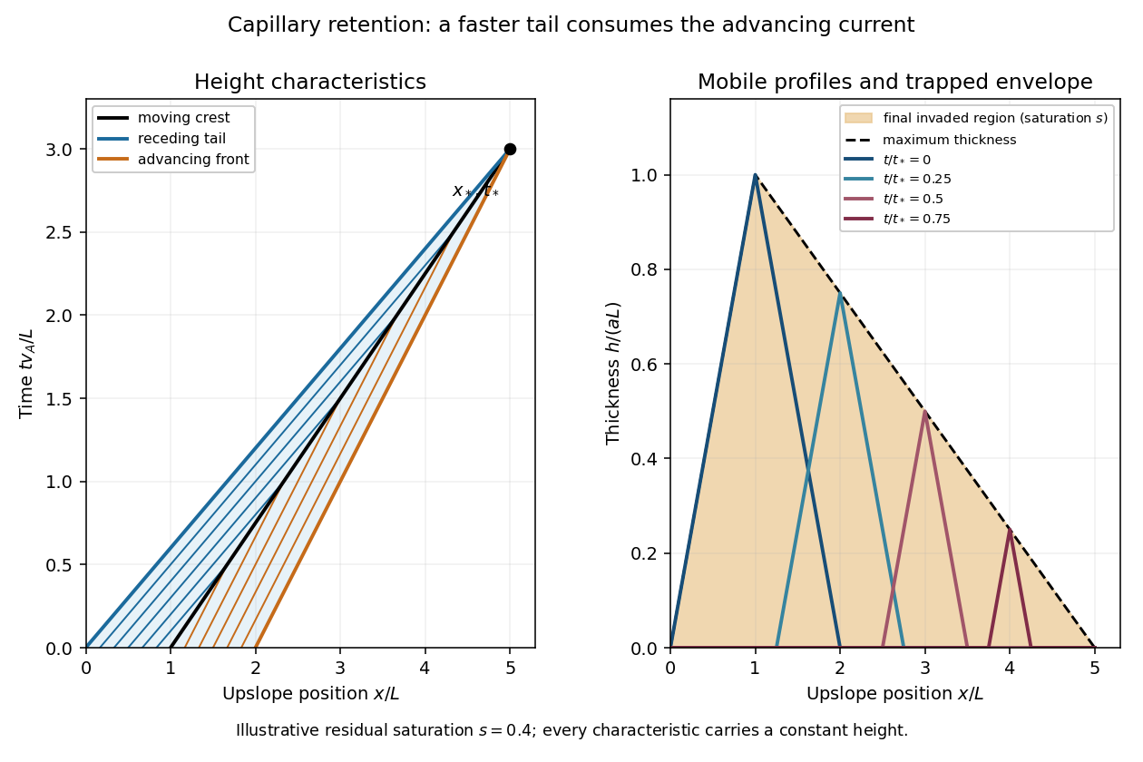
Advancing and receding characteristics, shrinking mobile profiles, and the final capillary trapping envelope
. The final trapped region is the maximum-invasion envelope of a retained current. For , the initial height is already the maximum, . For , the maximum occurs when the crest passes , at . Substituting into the trailing profile givesIf is distance into the aquifer measured normally from its upper boundary, trapped carbon dioxide occupies at residual pore saturation . The occupied pore volume per unit transverse width isexactly the initial mobile volume. This is an independent mass-conservation check of both the envelope and extinction distance. In the limit , the current translates without shrinking and nothing is trapped; the finite-extinction formula is not used in that limit.
Write for the positive reduced gravity of dense fluid. With upwards, places denser fluid above lighter fluid and permits convective turbulence. A displacement over the radius scale samples a buoyancy difference of order ; balancing kinetic energy per mass with buoyant work over givesThe buoyancy-gradient mixing-length closure then gives an eddy diffusivity . We use the paper's unit-prefactor convention for this dimensional closure and its effective cross-sectional area ; order-one mixing constants and the cylinder's geometric factor are suppressed in its displayed evolution equation.
The downward reduced-gravity transport magnitude and its convergence are different quantities:The printed expression labelled a flux is actually the second quantity, a flux convergence per unit height. The dimensions distinguish them: has units , whereas has units . A constant positive gradient has nonzero transport but zero convergence, providing a direct counterexample to identifying the derivative with the transport itself.
The upward total buoyancy flux is . Conservation therefore yieldsThis flux convergence in turbulent buoyancy mixing obtains the displayed evolution equation with the correct transport interpretation.
For the arrested cubic buoyancy profile, an undisturbed region below has and no turbulent buoyancy flux. The joining condition is andIn a steady state, integrating the conservation equation from that front gives . For a nonzero mixed region,and henceThe associated gradient is , so it matches the required zero-gradient state continuously. We take the mixed interval to start immediately above ; adding a further zero interval would merely relocate the arrest front.
The source buoyancy flux is , with in the Boussinesq approximation. The stated top-source convention means that this entire flux enters the downward turbulent transport there: . Since steady transport also satisfies ,This is the extent in the paper's dimensional-closure normalization. It presupposes positive ; with no upflow there is no finite steady arrest depth. For a mixture of the two original fluids, is necessary, so an extrapolation to cannot represent a physical concentration profile under this top-flux boundary model. A dilute-source regime avoids appreciable source-volume corrections.
Assuming the same scalar-mixing coefficient for a passive tracer, its eddy diffusivity in the mixed region isIt vanishes at the arrest front and increases linearly towards the source. A different turbulent scalar diffusivity ratio would multiply this result by its corresponding constant.
The geometric normalization can be restored without changing the reasoning. With actual area and , put . Then , , and . These formulas show which numerical prefactors are convention-dependent.
Use the well-mixed natural ventilation model for a distributed floor source. Let the building height be , its volume be , its temperature excess be , and the exterior mass density be . Let be the coefficient of thermal expansion, so reduced gravity is . Convert the total heat input to the temperature-volume flux , where is specific heat capacity. If the quoted heat flux is per floor area, first multiply it by that area.
For effective opening area for pressure-driven ventilation, define the equal-opening hydraulic coefficient such that the signed throughflow obeys , with the total driving pressure divided by mass density. In the effective-area convention of question 6, each opening has discharge , so . The usual physical-area orifice law instead gives ; that prefactor does not affect the stability conclusions.
Set and . Positive denotes entry at the floor and exit at the roof. hydrostatic pressure and wind combine to giveBecause the inflowing air is at exterior temperature in either direction, the heat budget isThe well-mixed ventilation temperature balance at steady state is thereforeAll roots must satisfy and their appropriate flow-direction inequality; squaring a pressure relation without imposing those conditions could add spurious branches.
The assisting case has a unique positive solution and it is stable. For opposing wind, define . There is always one solution with , a buoyancy-dominated upward flow. Below , the heat-removal curve is . It is zero at both endpoints, and its maximum occurs at :For there are two downward-flow roots as well as the upward-flow root. Equivalently, setting and , the equilibrium curve isFor linear stability analysis of the opposing-wind ventilation bistability, linearize the heat budget: the eigenvalue is . The cooler downward root has and , so it is stable. The warmer downward root has and , so it is unstable and separates the two basins. The upward root has and is stable. At the two downward roots merge at a saddle-node bifurcation; above that value only the upward equilibrium remains.
For ventilation switching under wind and heating changes, increasing wind pressure or decreasing heat input both reduce , so both can create the pair of wind-driven equilibria. They nevertheless have different physical and transient effects. On the hot upward branch, implicit differentiation of shows that increasing increases , while decreasing decreases . Both reduce the upward ventilation rate, but only a wind change shifts .
Under slow parameter variation, a state follows its current stable branch while that branch persists; the upward branch does not disappear when wind increases or heating decreases. A sufficiently large abrupt wind increase can raise beyond the current temperature and place that state below the new unstable threshold, causing flow reversal and cooling towards the wind-dominated equilibrium. A jump insufficient to cross its basin boundary returns to the upward equilibrium.
At fixed , reducing a still-positive heat input cannot force an initially upward-flow state through : at that boundary the temperature balance has . Thus heat reduction alone does not cause that reversal in this model. Conversely, decreasing wind or increasing heat from the stable downward branch eventually destroys it at the fold and forces a switch to the upward branch, giving history dependence. Wind strengthening and heat reduction have the same effect on the steady dimensionless control parameter, but not the same temperature change or switching dynamics. These stability statements use quasi-steady opening flow and a single well-mixed temperature; other stratification or airflow-inertia models require their own stability analysis.
Let be floor inflow and roof outflow. Use effective-area discharge , matching the factors in the supplied relations. With negligible source volume, both equal . The lower region has exterior mass density while the warm upper layer has reduced gravity and depth . hydrostatic pressure therefore supplies a total opening pressure head . Equal openings sharing equal discharge take half each, givingSteady lower-layer volume conservation sets this ventilation rate equal to the entrained turbulent plume flux at the interface, . Upper-layer buoyancy conservation gives . These are the required balances for displacement ventilation:Eliminating and gives the displacement-ventilation interface height equationThe left side is strictly increasing from zero to infinity, so there is one interface height. It depends on opening geometry and plume entrainment, not on ; the resulting and throughflow do depend on .
For finite source volume , conservation instead gives . The two pressure drops are no longer equal:Let be a physically entraining source plume: and for . Its interface balance is . Therefore, as reaches zero, a positive-depth lower layer has no replenishment and cannot remain steady: this is no steady displacement layer without ambient supply. The limiting interface is . At the threshold and , and the entire hydrostatic head drives the roof discharge. HenceThis is source-volume blocking of displacement ventilation. The half-head factor of the negligible-source state must not be kept after the floor inflow vanishes. In the usual physical-area convention , the equivalent formula is .
The quoted pure-plume law cannot be used unmodified down to the origin for a source with nonzero volume: it would incorrectly give zero flux there. A compatible finite-source example uses a virtual origin,It recovers the supplied pure-plume limit when , and gives the same blocking threshold. The complete finite- interface trajectory depends on that plume model, but the threshold needs only source-volume conservation and positive entrainment. For , the assumed steady regime with a lower inflow no longer exists.
Articles by others on the same topic
There are currently no matching articles.