An acoustic analogy is an exact rearrangement of the fluid equations into a chosen linear propagation operator acting on an acoustic variable, with everything left over placed on the right as effective forcing. The rearrangement becomes a sound-prediction method only after a reference medium, boundary conditions and approximations to the forcing are specified. In particular, a right-hand-side term need not represent independently generated sound.
Use Einstein summation convention and write . Differentiating the continuity equation in time and taking the divergence of the momentum equation eliminates :Set and . Since , the constant has zero Laplacian. The prescribed reference mass density and reference speed of sound are independent of time, soCombining the two identities givesOnly conservation of mass and conservation of momentum have been used; no equation of state or energy equation was needed. Spatial variation of creates no omitted derivative in this identity, because it multiplies a time derivative. The double divergence of the momentum flux tensor has the structure of an acoustic quadrupole.
For a localized flow, choose the reference fields to match the stationary surrounding medium: and outside the flow, with chosen so there. A uniform surrounding fluid permits ambient constant mass density and adiabatic sound speed, giving the familiar homogeneous wave equation. A nonuniform surrounding fluid calls for its actual stationary reference profiles, extended sensibly through the flow region. This makes the acoustic variable vanish in the unperturbed exterior and minimizes artificial contrast terms. In a uniform isentropic exterior the leading acoustic relation also makes vanish to first order. In a stratified exterior, propagation and entropy-advection effects can remain in , as the next part demonstrates.
At rest, all time derivatives and advective terms vanish. The continuity equation and the stated energy equation are then identities, while the momentum equation reduces to . The reference state need not have uniform mass density or entropy. Assume smooth positive reference pressure and mass density, and retain only first-order perturbations.
The linearized continuity equation, momentum balance and adiabatic energy relation areThe perturbation of multiplies a vanishing reference material derivative, so it does not enter at first order. Differentiate the last equation in time, then substitute the linearized momentum equation:Expanding the divergence yields the stratified acoustic pressure equationFor a perfect gas, . Put . ThenThus the divergence-form stratified acoustic pressure equation isThis is homogeneous linear propagation through the static medium, including its inhomogeneity. In the acoustic analogy of part (a), has no first-order contribution when viscosity is neglected and the reference velocity is zero. Nevertheless the chosen left-hand operator lacks the gradient terms in the genuine propagation equation. Those effects must consequently appear in . They describe propagation of an existing disturbance, rather than an independent source. Since reference-field choices also change the division between the operator and forcing, cannot be identified unambiguously with newly generated noise. Its presence in the right-hand side is a consequence of the chosen analogy, not a source-classification theorem.
Retain from part (b), and use time translation invariance to write . Define the temporal Fourier transform byMultiplying the transformed Green function equation by givesThis is a symmetric divergence-form spatial operator, although the original unweighted operator need not be symmetric in the ordinary volume measure.
Let . The product rule gives the bilinear Green second identityThe frequency terms cancel. Integrating over the domain, the right side becomesThe boundary integral is zero for common homogeneous Dirichlet boundary condition, Neumann boundary condition or reciprocal Robin boundary condition conditions. In an unbounded domain, use the same outgoing limiting-absorption prescription for both Green functions; it gives the corresponding vanishing boundary pairing. This identity has no complex conjugation: it proves transpose wave reciprocity, not a Hermitian or time-reversal identity. We obtain the weighted acoustic Green-function reciprocityThe factor is frequency independent, so inverse Fourier transform gives the same relation at equal time lag. Both time arguments below have lag , henceReciprocity exchanges source and receiver while preserving elapsed time; it does not turn a causal response into an advanced one.
Suppress the common time factor , take , and fix the spatial Fourier transform conventionA plus transform is supported on and analytic above ; a minus transform is supported on and analytic below it. For the outgoing radiation condition with this time convention, initially take , , and pass to the limit at the end. Thus lies below the contour and above it.
Choose to have positive real part on the real transform line. Its branch cuts run from into the lower half-plane and from into the upper half-plane, without crossing ; downward and upward vertical rays are suitable. In the zero-absorption limit, for real and between the branch points. This ensures that represents decay or outgoing radiation, rather than an incoming exterior field.
Evenness in and the Helmholtz equation give the transformed fieldsAt , the one-sided normal derivatives of the scattered field agree for , because that part of the interface is open. For they both vanish by rigidity. Their common trace is therefore a minus function, denoted . ConsequentlyThe jump in the total scattered transform isFor , continuity of the total mass density requires the scattered jump to cancel the incident jump, so . Its minus transform is . The unknown plate-side jump is the plus function . Thus , and the Wiener-Hopf equation follows:
Use the Wiener-Hopf factorization , with factors analytic and nonzero in their designated half-planes. Their analytic continuations allocate outgoing modal zeros to below the contour, and the opposite zeros to above it. Set . Multiplication by and pole subtraction giveThe pole in the upper expression is removable by its numerator. The two expressions analytically continue to the common entire function, which is zero under the stipulated edge/growth assumption. Henceand the transformed fields areA constant reciprocal rescaling of the factors does not alter or the physical field.
Inside the guide, and are even entire functions of , while is analytic in the lower half-plane. Thus continuation across the lower branch cut changes none of the interior transform: that cut is removable. The exterior expression retains the cut, corresponding to radiation into the open exterior.
For , the inverse-transform contour closes downwards, clockwise. Away from modal cutoffs, its enclosed singularities are the outgoing simple poleswith positive real part for propagating modes and negative imaginary part for decaying modes; is the root. The opposite roots lie above the contour or cancel against zeros of . Symmetry excludes odd transverse modes. At , , and differentiation of givesEach inverse-transform contribution is times its residue. Therefore the outgoing modes of an open rigid acoustic waveguide areThe original time factor multiplies this expression. Thus every cut-on mode propagates in the positive direction; cut-off modes are evanescent waves decaying into the guide, not additional backward waves. Strictly, a complete mode sum includes these evanescent modes as well as propagating ones. The displayed simple-pole amplitudes apply away from exact cutoffs; cutoff values use the outgoing limiting-absorption continuation before taking the limit. The reflected plane-wave amplitude relative to the unit incident wave is above. It has the expected negative sign in the long-wavelength leading kernel approximation .
Write the negative-flux Inviscid Burgers equation as , with . Along a characteristic curve,so a characteristic starting at has andThis formula is a classical solution only while the method of characteristics is one-to-one; after characteristic crossing one must select an entropy solution.
For a discontinuity with left and right values and , the Rankine-Hugoniot condition follows by integrating conservation across a moving small interval:For a nonzero jump, factor the difference of squares to obtainThe negative flux makes increasing jumps compressive. Decreasing jumps spread into rarefaction waves; they cannot be retained as nonphysical expansion shock waves.
In the central ramp of each period, , so its method of characteristics is . For , the retained ramp therefore occupies . At the odd boundary , the initial limiting values are on the left and on the right. Their characteristic speeds are and , giving the fan on . Together these give the periodic backward-sawtooth Burgers solutionThese intervals tile the real line up to their matching endpoints, where both formulas agree at . The increasing ramp steepens, but the wave's maximum magnitude remains one before breaking. A steep continuous regularization of the original downward jump produces exactly the limiting fan, as suggested by the characteristic construction.
At , each increasing ramp collapses at . The fans on either side meet there with values and , producing a compressive stationary shock wave. For all the fan between successive shock waves remains centered at the odd point, givingAt a shock wave the limiting values are and . Their average is zero, so the Rankine-Hugoniot condition keeps the shock wave fixed. Their characteristic speeds satisfy , confirming compression into the shock wave. The arbitrary pointwise value at a shock wave does not affect the weak solution. The post-breaking amplitude decays as , despite the lack of explicit viscosity, because shock wave dissipate the wave.
For the requested sketches, has ramp slope on and fan slope around odd points on width . It is still continuous. At , the profile decreases linearly with slope between even points and jumps from to at each even point:
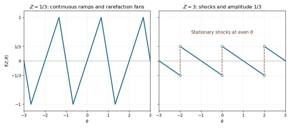
Periodic Burgers wave before breaking at Z equals one third and after breaking at Z equals three, with stationary shocks at even theta
. Details. 
Let , with , and set . Direct differentiation givesThe heat equation implies , so the bracket vanishes. Conversely its being independent of can be absorbed into a -dependent multiplicative normalization of , leaving unchanged. This proves the Cole-Hopf transformation with the positive sign appropriate to the negative-flux Burgers convention. Although the algebra works for nonzero , the given forward Gaussian function diffusion kernel and a physical vanishing-viscosity limit require .
Take for the stated Burgers N-wave. Integrating and normalizing the exterior value to one givesThis function is continuous at ; its logarithmic derivative has the specified jumps. Convolution with the heat kernel is positive and solves the heat equation for . Splitting the integral into the exterior baseline and the interior correction yieldsPut . Completing the square givesChanging the interior integration variable to changes its limits to and the Gaussian function width to . The Jacobian and normalization leave the factor . Thus the Cole-Hopf solution for a Burgers N-wave isHere is the normalized Gaussian function mass of its indicated interval. Its explicit error function representation isFor fixed , the Gaussian function concentrates at as . Consequentlyaway from the endpoints; at the limit is . The transition layer has width . This is an approximate identity argument, not a uniform step approximation across the endpoints.
For fixed and , both interval masses tend to one, and the exponentially large positive dominates the exterior correction. Its logarithmic derivative therefore givesFor , both interval masses are exponentially small and the weighted interior integral is also negligible, while the exterior contribution tends to one. Therefore in the specified far exterior.
An exponentially weighted Gaussian function tail should not be discarded solely because its unweighted interval mass tends to zero. In fact, comparing the order-one exterior term with gives the sharper inviscid Burgers N-wave fronts , not . Away from these fronts, the vanishing-viscosity limit isInside , this follows from the sign of in the exponential. Outside , the constrained Gaussian function maximum lies at an interval endpoint and has negative exponent. The right shock wave's speed is , equal both to the derivative of and to minus half the sum of its two limiting states; the left shock wave is its reflection. This checks consistency with the Rankine-Hugoniot condition and shows that the requested near-center and far-exterior approximations are compatible with the full entropy limit.
Articles by others on the same topic
There are currently no matching articles.