Use inverse temperature , reserving without a subscript for the critical exponent. Write ; each undirected bond occurs once, so the number of bonds is . In the mean-field theory of the Ising model, write each Ising spin as and neglect the product of fluctuations:The resulting independent-spin statistical Hamiltonian isThe constant corrects the double counting of interaction energy. The Ising spin sums now factorize and can all be evaluated:This is the approximate partition function at an assumed mean field; equilibrium fixes self-consistently. The corresponding Ising auxiliary mean-field free energy isIts equilibrium value gives the mean-field Helmholtz free energy in the imposed field. Away from a stationary point its parameter is an assumed field variable, not necessarily the actual mean Ising spin of that independent-spin distribution.
For the full small- expansion at fixed , set and . Differentiating gives successive derivatives , , , and at . ThereforeAt zero field, spin inversion symmetry eliminates odd powers and this simplifies toThe quadratic coefficient changes sign and the quartic coefficient is positive atThus the zero-field mean-field prediction is a continuous, continuous phase transition: the stable zero spin magnetization develops two symmetry-related nonzero minima continuously below .
Both requested routes give the same mean-field self-consistency equation. First, the one-spin expectation in the effective field isSecond, differentiating the Ising auxiliary mean-field free energy giveswhose stationary condition is precisely that mean-field self-consistency equation. Choose its stable, lowest-free-energy branch rather than every algebraic solution.
An equally useful mean-field approximation parametrizes the trial distribution by its actual mean Ising spin. Its probabilities are , giving the Bragg-Williams free energy of the Ising modelThis energy-minus-entropy function has expansionIts stationary equation is , again equivalent to the mean-field self-consistency equation. The two functions differ away from equilibrium, but agree on stationary branches: for and , the entropy bracket equals . Their small- coefficients therefore need not agree at arbitrary temperature; at they have the same leading critical quartic coefficient . This distinction prevents confusing the auxiliary-field expansion with the physical-magnetization variational expansion.
For the order-parameter critical exponent, expand the equation of state at :On a nonzero stable branch,Hence . The spontaneous magnetization is understood by selecting a branch with an infinitesimal field after the thermodynamic limit; a finite symmetric sample has zero exact zero-field mean Ising spin.
For the magnetic susceptibility per site, define with in energy units. Implicit differentiation givesAbove , and . Below , evaluated on a selected ordered branch, the expansion of gives . Thus the magnetic-susceptibility critical exponent is on both sides, with different amplitudes. At , the equation of state becomesso the critical-isotherm exponent is . These are mean-field critical exponents, not a claim that neglecting fluctuations gives the exact Ising transition in every dimension.
Assume the scalar order parameter can take either sign. The cubic term breaks symmetry, and a positive quartic coefficient bounds the Landau free energy below. Stationary points satisfyso, besides the disordered point , the possible ordered points areThe disordered point has curvature and is locally stable when . Nonzero stationary points first appear whenThat condition alone does not make them the equilibrium phase: one must compare their free energies.
At a nonzero stationary point, substitute to obtainFor an ordered state to coexist with , this requiresBoth curvatures at phase coexistence are positive and equal to . The barrier is at . In fact the potential at phase coexistence factorizes:The two distinct minima are therefore explicit, with a finite jump in the order parameter whenever .
To state the equilibrium inequalities for either sign of , put with . This sign always has lower energy than the opposite sign of equal magnitude. ThenThe bracket's minimum is . It follows thatThe favored ordered minimum, when it exists, isThus a first-order phase transition is possible and occurs when the coefficients cross the coexistence relation. There is no continuous transition between and the equilibrium ordered state while remains nonzero and remains finite and positive. The ordered state becomes globally favorable while is still positive, before the disordered curvature can vanish. Although a stationary solution tends to zero at , it is not the global transition branch. A continuous transition would require eliminating the cubic term, outside the stated condition.
The spinodal points clarify the metastable region: for the ordered minimum is metastable; for the disordered minimum is metastable. At the disordered state loses local stability. These local-stability limits should not be mistaken for the first-order transition in a cubic-quartic Landau potential.
Use dimensionless interaction couplings in the exponent of the Boltzmann weight. In the following formulas denote the physical interaction energies divided by if that factor has not already been absorbed into the displayed Hamiltonian. This convention is required for temperature-independent numerical fixed-point coordinates.
Split the original square lattice into retained sites with even and eliminated sites with odd , where coordinates are in units of . Every nearest-neighbour bond joins to , whereas a diagonal next-nearest-neighbour bond stays within one sublattice. Denote retained Ising spins by and eliminated Ising spins by . For fixed retained Ising spins defineThe blocked Boltzmann weight in the checkerboard decimation of the square-lattice Ising model isUse the independent uniform product measure on Ising spins on to perform a cumulant expansion. Its one-spin mean vanishes, and . Consequently the first-order term, the first-order eliminated-sublattice term, and the mixed term vanish. To the requested order,Here the truncation keeps and the linear term in ; equivalently count as order . At higher orders the interaction family will generally not close.
Each eliminated site has four retained neighbours, soIts six distinct neighbour pairs comprise four corner pairs at distance and two opposite pairs at distance . A given retained diagonal pair shares two eliminated centres; a given opposite pair shares only one. Thus the generated pair couplings are for diagonal pairs and for axial pairs separated by two original spacings. The original interaction directly contributes to each retained diagonal pair. No single-spin term survives spin inversion symmetry, and no three-spin or four-spin term is present in this second cumulant. This proves closure on exactly two nonconstant interactions at the retained order.
The primitive vectors of the retained square lattice are and . Rotate the axes by degrees and rescale lengths by ; retained diagonal pairs become nearest neighbours, and the axial distance- pairs become next-nearest neighbours. With , the leading checkerboard Ising decimation recursion is thereforeThe constant part of the weight is also determined: , so the original partition function equalsto the same order in the logarithm of the weights. That normalization changes free energy but not the retained-spin interaction operators. If physical energy couplings are kept instead, at fixed the relations read and .
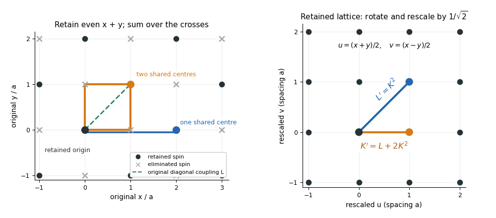
Two shared eliminated neighbours generate a nearest-neighbour bond; one generates a next-nearest-neighbour bond after checkerboard decimation
. Details. 
The fixed-point equations are and . Their only finite real solutions areThe origin is the high-temperature fixed point; its Jacobian matrix is , with both multipliers zero. The nontrivial candidate critical point is . Linearize the discrete renormalization-group transformation there:The characteristic polynomial is , givingEigenvectors may be chosen as . The positive eigenvalue greater than one is the relevant direction of a fixed point; the other is irrelevant because its magnitude is less than one. Its negative sign only alternates the sign of the perturbation between steps. For a discrete map the magnitude relative to one decides relevance, not the sign rule used for continuous beta-function eigenvalues.
Let be the relevant thermal scaling coordinate, so to first order. A correlation length measured in restored lattice units satisfies . If , then . Hence the thermal exponent from a discrete renormalization map isThis is the value predicted by the stated low-order real-space renormalization group, whose nontrivial fixed point is evaluated beyond the strictly infinitesimal-coupling limit. It is an approximation, not an exact solution of the full square-lattice Ising model.
The statistical Hamiltonian in this question is already in thermal units, as indicated by without an additional . Define and . The mean field and its linear response areThese are functional derivatives of the connected generating functional; the subtraction defines the connected correlation function. In the Landau approximation, neglect loop corrections and evaluate the field integral at a stable saddle . It satisfies the Euler-Lagrange equationThis follows by varying the gradient term and integrating by parts, with periodic, decaying, or otherwise appropriate boundary conditions.
The two requested free energy functionals, following the source and Legendre conventions of the question, areIn the scalar-field source Legendre transform on the chosen stable branch, is chosen to produce , and . Thus the imposed-source Helmholtz free energy and the fixed-order-parameter Gibbs free energy have the appropriate opposite source derivatives. These names are used in the question's magnetic-ensemble convention; the defining sign relation is what fixes the calculation. At leading Landau approximation there is no fluctuation-determinant term in .
Differentiate the saddle equation with respect to . The response obeysThereforeEquivalently, the inverse Hessian relation for a connected two-point function states that is the inverse kernel of . The factor follows from twice differentiating the quartic term ; it is not . This tree-level connected response is obtained by varying the saddle. It does not require replacing the exact connected correlator by a product of the saddle values, which would incorrectly give zero.
For the requested single-momentum formula, assume a homogeneous source and a translationally invariant equilibrium phase, so and . SetThe Fourier transform with the printed positive sign sends to , while the Dirac delta function transforms to one. Hence the Ornstein--Zernike correlation function hasThe inverse convention is . For general inhomogeneous , has nonconstant coefficients and depends separately on its two positions; the displayed momentum-diagonal formula then does not follow. The preceding differential equation still holds in that case.
At zero source and for , the homogeneous saddle is for , and on either selected stable ordered branch for . Thus the Landau scalar correlation length isIn the ordered phase the negative bare quadratic coefficient is compensated by the positive curvature at the nonzero saddle. Retaining below the transition would instead give an unstable kernel and is not a physical correlation length. With the usual analytic thermal tuning , , both branches diverge as , so the correlation-length critical exponent isThe high-temperature amplitude is times the low-temperature amplitude for the same . This statement is within Landau theory; fluctuations can change critical behavior outside the mean-field regime.
When , the field theory is a Gaussian field theory, so integrating out short-wavelength modes can be done exactly rather than merely at a saddle. Introduce an ultraviolet momentum cutoff and a scale factor , then split into and . Orthogonality of Fourier modes eliminates cross terms in the quadratic Hamiltonian. A constant source couples only to the zero-momentum mode and therefore does not couple to .
Before rescaling, the Gaussian functional integral factorizes:where has the original and , restricted to low momenta. Up to a field-independent normalization, the eliminated modes contributeThe determinant affects the additive free energy, but generates neither a mass correction nor a source correction, since no interaction mixes low and high modes. This remains true beyond the Landau approximation: it is an exact integration of a Gaussian field theory, not neglect of the high-mode fluctuations.
To restore the original cutoff, use , , and choose the field rescalingSubstitution into the low-mode Hamiltonian gives the Gaussian momentum-shell scalingThe gradient coefficient is unchanged: the volume factor is , the two derivatives contribute , and the two fields contribute . The mass term gains , while the source term gains . ThusFor a nonconstant source the corresponding formula is , after restricting its coupling to retained modes. The constant-source case avoids that extra source filtering.
Writing , the exact Gaussian renormalization-group flow hasBoth perturbations are relevant at the massless zero-source Gaussian fixed point, with and . There is no anomalous field rescaling here, so and the correlation-length critical exponent is again . The coefficient changes arise from rescaling, not from an interaction-induced shift in during shell integration.
A stable real Gaussian functional integral requires , or an infrared prescription that treats the zero mode at the massless point. With and , the field energy is unbounded below; the Gaussian field theory alone cannot describe a stable ordered phase. The scaling laws are therefore interpreted about the Gaussian fixed point from the stable side, with finite-volume zero-mode regularization when needed.
Articles by others on the same topic
There are currently no matching articles.