Past exam of the physics of the Earth as a Planet course of the University of Cambridge / 2015 / Paper 1 / 1

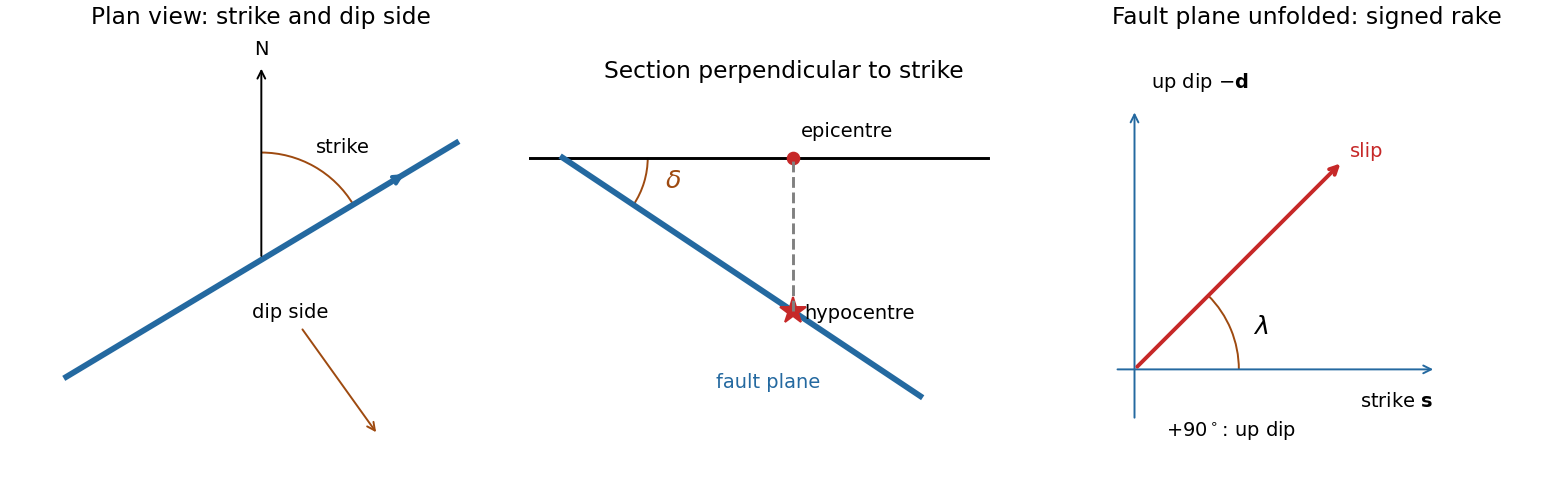
A fault plane represents the surface across which the two sides of a fault slip. A real fault need not be perfectly planar; these angles can describe a local planar segment. Its fault strike is the azimuth, measured clockwise from north, of its horizontal intersection. The line itself has a $180^{\circ }$ ambiguity; choose the direction for which the fault dips to the right. Its fault dip, $\delta$, is the angle below horizontal measured perpendicular to that fault strike, from $0^{\circ }$ for horizontal to $90^{\circ }$ for vertical.

The fault rake, $\lambda$, is the angle of the relative slip vector within the fault plane. State the sign convention: if $\mathbf{s}$ is the chosen strike direction and $\mathbf{d}$ points down dip, useThus $\lambda =0$ is slip along $\mathbf{s}$, $+90^{\circ }$ is up-dip slip and $-90^{\circ }$ is down-dip slip. This distinguishes the direction in which the fault is tilted from the direction in which it actually moves.

The hypocentre is the point where rupture begins within the Earth. The epicentre is the point on the surface directly above it. The hypocentre need not coincide with the centroid of the final rupture. Orientation uses strike and dip; motion additionally needs rake; epicentre and hypocentre locate the rupture's start.^[ref]

Assume a stable, lossless elastic body with the usual symmetry of the elasticity tensor and boundary conditions that eliminate the surface terms in integration by parts, such as a traction-free outer surface. Its elastic stiffness operator is then self-adjoint. When density varies spatially, the precise eigenproblem is generalized:Here $\alpha$ abbreviates the pair of mode labels. Equivalently, ${\rho }^{-1}\hat{H}$ is a self-adjoint operator in the mass inner product. Stability makes ${\omega }_{\alpha }^2$ real and nonnegative. Modes at different eigenvalues are orthogonal, and an orthonormal basis can be selected within each degenerate eigenspace. Completeness permits expansion of a suitable displacement field in these mass-weighted elastic normal modes.

Insert the expansion and project onto ${\mathbf{u}}_{\alpha }^{\ast }$. Mass normalization diagonalizes both the acceleration term and the restoring term. For a symmetric stress glut tensor supported away from the boundary,The symmetry of the stress glut tensor removes the antisymmetric part of the displacement gradient, leaving the strain. The result is one independent forced oscillator per mode, with the stated excitation integral. If the modes instead have mass norm $N_{\alpha }$, that integral is divided by $N_{\alpha }$. A source touching the boundary requires the corresponding surface forcing to be retained rather than silently dropping it.

Rigid translations and rotations can be zero-frequency modes of a free body. Their strain vanishes, so an internal symmetric seismic moment tensor does not excite them through this coupling. Attenuation, radiative boundaries or other non-self-adjoint effects require modifications of the simple conservative expansion.

For a mode of positive frequency, differentiation of the causal convolution givesThe first boundary term vanishes because $\sin 0=0$; the second supplies $f(t)$ because $\cos 0=1$. Both initial values vanish. This verifies the forced-oscillator equation and its initial conditions, including a step source in the piecewise or distributional sense.

The spatial Dirac delta function reduces the excitation toFor an event at $t_s\ge 0$, put $\tau =t-t_s$. Integrating the oscillator kernel from $t_s$ to $t$ gives the normal-mode response to a step seismic moment:Non-unit mass normalization introduces the same factor $1/N_{\alpha }$ as above. Complex modes must be combined with their conjugate partners to produce a real displacement. The formal $\omega \to 0$ limit is $a=C{\tau }^{2}H(\tau )/2$; for rigid-body modes here, $C=0$ because their strain is zero.

The step produces a static component plus continuing oscillations in this lossless model. It does not predict physical damping. A point source is appropriate when rupture dimensions are small compared with the wavelengths being analysed and rupture duration is short compared with their periods. Long-period observations of a relatively small earthquake can meet these conditions; high-frequency finite-fault directivity generally cannot. A finite source-time function replaces the ideal instantaneous step when its duration matters.

For seismic source inversion, collect calibrated, consistently filtered samples from all available stations and components into a data vector $\mathbf{d}$. For each trial source position and origin time, compute the corresponding elastodynamic Green tensor in an Earth model, including the instrument response used for the data. Write the symmetric seismic moment tensor in six independent symmetric basis tensors:Each column of $\mathbf{G}$ is the synthetic seismogram for one basis tensor. An off-diagonal basis tensor contains both symmetric entries, so the double contraction and its factors of two remain consistent.

A suitable objective iswith noise covariance ${\mathbf{C}}_d$; a justified penalty can be added for regularization. At fixed $\mathbf{q}$, solve for the six entries of $\mathbf{m}$ by weighted least squares, preferably using a QR decomposition or singular value decomposition rather than explicitly inverting the matrix of the normal equations. Then search over the four nonlinear parameters using a coarse location/time grid followed by local refinement. This variable projection reduces a ten-parameter search to a four-parameter nonlinear search with an inner six-parameter linear fit. Merely having more than ten data samples does not ensure identifiability: the design matrix must have adequate rank and the network must resolve the source's radiation patterns.

Potential errors include inaccurate velocity, density, anisotropy and attenuation in the assumed Earth model; neglected finite rupture and source-time effects; timing, instrument calibration or component-orientation errors; correlated noise; uneven station coverage; and tradeoffs between depth, origin time and the moment tensor. Imposing a double-couple seismic source mechanism without evidence can hide genuine non-double-couple components. Regularization also changes the recovered source and should be reported.

Inspect residuals, singular values, recovery of synthetic sources and uncertainty under resampling or noise perturbations. Linearized covariance or a posterior distribution can quantify uncertainty within the assumed forward model, but does not automatically account for errors in that model. A good waveform fit alone is insufficient evidence that all ten parameters are uniquely recovered.