gravity and surface topography. gravity responds to all density structure, while surface topography records both load and support. First specify the reference field and measurement height. latitude and planetary rotation affect normal gravity. At elevation , the reference field decreases approximately by ; a free-air gravity anomaly restores this elevation effect but retains topographic mass. A Bouguer gravity anomaly additionally subtracts an approximate topographic slab contribution . terrain correction replaces the unrealistic slab near valleys and ridges, and spherical geometry matters over large areas. A density choice is required for these reductions; a numerical crustal density is not provided here.
In Airy isostasy, surface topography of height and crustal density is compensated by a root of thickness replacing mantle of density . Equal column masses give . The positive gravity of the relief is partly cancelled by the negative density contrast of the root. At long wavelengths a compensated mountain can therefore have a modest free-air anomaly and a negative Bouguer anomaly. Pratt isostasy instead varies column density at a roughly common compensation depth. Neither model says that surface topography itself exerts no gravity.
Potential-field depth filtering makes wavelength crucial. In a planar Fourier approximation, a density interface at depth is attenuated by at horizontal wavenumber . For a small Airy-compensated height perturbation and a compensation interface at depth , the gravity-topography admittance is approximatelyLong wavelengths allow strong cancellation between load and root. At short wavelengths the root's gravity is filtered out, so the observed near-surface mass can dominate even if the column is compensated. In a flexural isostasy model, an elastic lithosphere supports and spreads the load; for downward deflection and imposed load , , with . Thus , and the effective elastic thickness controls the support scale.
Estimate admittance from cross-spectra of gravity and surface topography, and compare its wavelength dependence and coherence with local-compensation, elastic-flexure and subsurface-load models. A primary Atlantic study sampled ship-track free-air gravity and bathymetry and compared their Fourier-domain relationship with compensation models, illustrating this observational route rather than inferring a root from the sign of one gravity value.[ref]
The relationship between bathymetry and gravity in the Atlantic Ocean by Dan McKenzie and Carl Bowin. pp. 1903–1915, ship-track sampling, spectral transfer estimates and wavelength-dependent compensation
Check navigation, instrument drift, terrain/density reductions, sediment and water loads, and independent seismic crustal constraints. Density-depth trade-offs and mantle dynamic support make the inverse problem nonunique; surface topography and gravity together constrain support, but do not uniquely map every density anomaly.mantle viscosity. A second, independent route concerns deformation rates rather than static compensation. glacial isostatic adjustment follows loading and unloading of a deformable Earth: an ice sheet depresses the surface, and subsequent removal leaves time-dependent uplift, horizontal displacement, sea-level and gravity changes. Fit dated relative sea-level indicators and raised shorelines together with geodetic displacement rates and a reconstructed ice/water load history to a viscoelastic Earth model. Relative sea level includes solid-surface motion, changing geoid and redistribution of ocean water; treating it only as local vertical rock motion biases the inference.
For scale, a sinusoidal surface perturbation of wavenumber on a uniform incompressible viscous half-space relaxes under gravity with . A Maxwell material separately has a stress-relaxation scale . These are different experiments and generally different times: rebound modes also involve gravity, spherical geometry, a layered mantle and elastic lithosphere. Fit a family of relaxation modes or a full load-history convolution, rather than equating every observed rebound time to .
Use independent ice-margin, exposure-age and sea-level constraints to reduce the trade-off between ice history and viscosity; compare horizontal as well as vertical GNSS motions, and separate present ice loss, groundwater changes and tectonic signals from the older loading response. A primary global analysis jointly tested ice-history and mantle-response predictions against space-geodetic observations, rather than treating a local uplift rate as a unique viscosity measurement.[ref]
postseismic relaxation probes shallower or faster relaxation after a stress perturbation, but must be distinguished from afterslip and poroelastic deformation. Long-wavelength geoid and mantle-flow models provide complementary constraints when density structure is estimated independently from seismic structure and mineral physics; unknown density-to-velocity conversion and boundary tractions remain trade-offs. Laboratory creep experiments constrain constitutive laws as functions of temperature, stress and grain size, but require a large extrapolation to geological conditions. Combine spatially and temporally distinct observations; there is no single directly measured mantle viscosity independent of depth, rheology and loading assumptions.
First-motion source mechanisms. Locate an earthquake from arrival times and use a seismic velocity model to calculate each station's source takeoff direction. Measure the initial direct P wave polarity after checking instrument sign, component orientation, timing and phase identification. An upward trace at an instrument is not automatically a source compression without the propagation and component convention. Plot the inferred source radiation signs on a focal sphere, commonly using a lower-hemisphere equal-area projection, and seek nodal planes separating positive and negative observations.
For a shear dislocation with orthogonal unit slip and fault-normal vectors , the double-couple fault source has . Its far-field P radiation sign is that ofThe two zeros are orthogonal nodal planes; the four quadrants alternate between outward and inward initial radiation. Their orientations and quadrant signs determine candidate strike, dip and rake. Normal, reverse and strike-slip mechanisms give different projected patterns. The earthquake pressure and tension axes are the negative and positive moment-tensor principal directions, respectively; they do not by themselves measure the complete regional stress tensor.
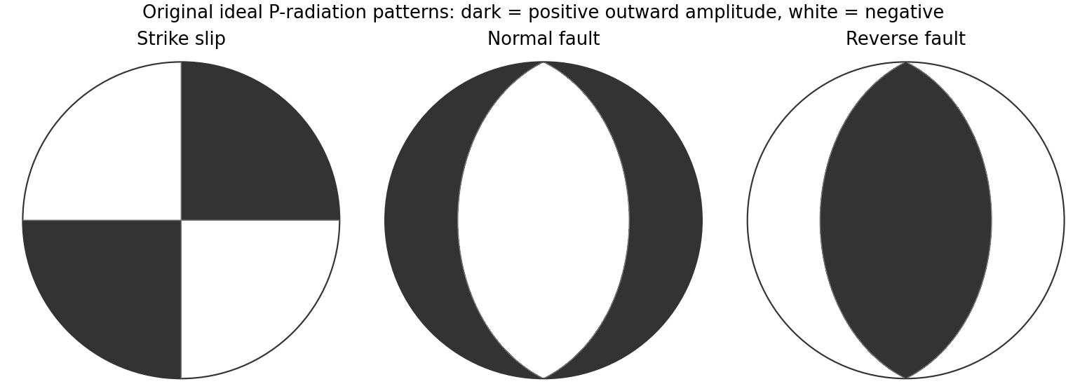
Original lower-hemisphere equal-area P-radiation polarity examples for ideal strike-slip, normal and reverse double couples
. Details. 
There is a fundamental fault-plane ambiguity: exchanging and leaves the radiation tensor unchanged. First motions therefore give a fault plane and an auxiliary plane without saying which actually slipped. Use mapped rupture, aftershock geometry or independent geodetic displacement to select the physical fault where possible. Polarity signs alone do not measure scalar seismic moment, source duration or rupture extent. A poorly sampled focal sphere or many near-nodal observations can admit several mechanisms rather than one defensible beachball.
Propagate uncertainty in event depth, velocity gradients and takeoff angles, allow for mispicked or reversed polarities, and report the range of mechanisms consistent with the observations. A primary method did this by testing alternative locations and velocity models and validated its uncertainty estimates using noisy synthetic data and clusters of events with similar waveforms.[ref]
A New Method for Determining First-Motion Focal Mechanisms by Jeanne L. Hardebeck and Peter M. Shearer. pp. 2264–2266 and abstract, first-motion construction, polarity/takeoff uncertainty and independent validation tests
Broadband waveforms and amplitude ratios add information, especially for non-double-couple sources, but they are additional measurements rather than a way to extract amplitude information from a sign-only data set.Radial density structure. In an isotropic adiabatic material, the seismic parameter isFor a chemically homogeneous region whose background stratification is adiabatic, . Combine this with spherical hydrostatic balance and mass conservation to obtain the Adams-Williamson equationsThe inward density increase follows compressibility under the increasing pressure. A specified starting density and measured allow integration within a homogeneous adiabatic layer. Seismic velocities alone, however, do not determine that density normalization, since they contain ratios of moduli to density. Chemical boundaries, phase transitions, nonadiabatic thermal gradients and anisotropy require additional modeling; a composition jump is not obtained by blindly integrating the smooth relation across it.
Use travel times and surface waves to constrain elastic velocities, reflected/converted phases to locate interfaces, and normal-mode frequencies to constrain density as well as elastic structure through their sensitivity kernels. Impose independently known total mass and moment of inertia:Because these weight depth differently, they help distinguish admissible profiles, but two integrals alone do not specify an arbitrary radial function. Laboratory equations of state and mineral physics restrict composition, compressibility and density jumps. pressure and enclosed mass are matched across interfaces, while density may jump. In a liquid region and , so the shear-wave absence constrains phase state without itself providing a direct density measurement.
The Preliminary Reference Earth Model is a concrete joint inversion of seismic travel times, normal modes, mass and inertia, including density and attenuation along with elastic structure. The original analysis combined these complementary data rather than deriving density uniquely from P wave speed.[ref]
Preliminary reference Earth model by Adam M. Dziewonski and Don L. Anderson. abstract and pp. 297–300, data classes and coupled radial reference-model inversion
A defensible radial density model combines hydrostatic/thermodynamic relations with seismic and global integral constraints, and states where homogeneity and adiabaticity fail. Articles by others on the same topic
There are currently no matching articles.