Past exam of the quantum matter course of the University of Oxford / 2025 / 2

Measure single-particle energy from the quantum harmonic oscillator ground state energy $\hslash \omega$, and write $\tilde{\mu }={\mu }_{\mathrm{physical}}-\hslash \omega \le 0$. The Bose-Einstein distribution and the supplied density of states giveThis excited-state population increases with the chemical potential and has the finite saturation valueAny additional particles must occupy the ground state: this is two-dimensional harmonic-trap Bose condensation. The critical temperature and the condensate fraction are thereforeHere $N$ is the total particle number, the integral of the inhomogeneous number density over the trap; there is no fixed uniform area in which $N$ itself is a number density. Equivalently $N\kappa ={\pi }^{2}m(k_B{T}_c{)}^2/(6{\hslash }^2)$ relates the trap population to the critical temperature. Harmonic confinement changes the low-energy density of states and permits this saturation in two spatial dimensions.

These formulas are leading large-$N$ results with $k_B{T}_c\gg \hslash \omega$. A sharp transition belongs to the trapped-gas thermodynamic limit $N\to \infty$, $\omega \to 0$ at fixed $N{\omega }^2$; a finite trap has finite-size rounding. In particular, finite $N_0$ requires $\tilde{\mu }=-k_{B}T\log (1+1/N_0)<0$, approaching zero in the condensation limit.

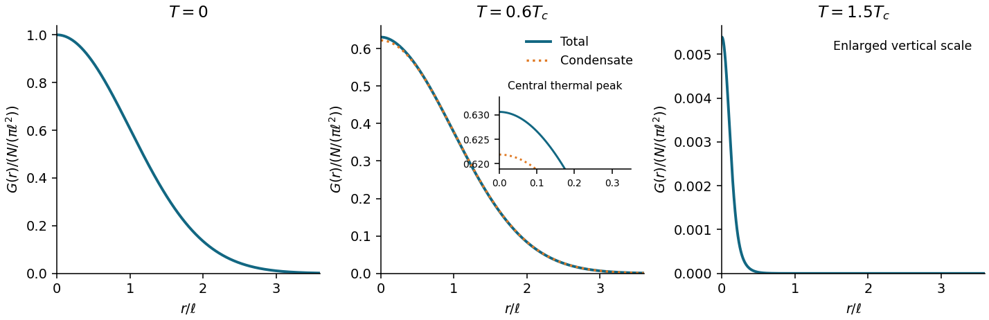
Write $G(r)=⟨{\psi }^{†}(0)\psi (\mathbf{r})⟩$, $r=|\mathbf{r}|$, and ${\ell }^2=\hslash /(m\omega )$. At zero temperature all $N$ particles occupy ${\varphi }_0(\mathbf{r})=(\ell \sqrt{\pi }{)}^{-1}{e}^{-r^2/(2{\ell }^2)}$. Expanding the bosonic annihilation operator in single-particle orbitals givesThis one-body density matrix is a Gaussian function of width $\ell$; it contains one wavefunction evaluated at $r$, so its exponent is half that of the spatial number density $N|{\varphi }_0(r){|}^2$. In particular,the total number density at the trap centre, including condensed and noncondensed particles.

At positive temperature, with occupations ${\overline{n}}_a$ of the trap energy eigenstates, the exact ideal-gas decomposition isFor $\hslash \omega \ll k_{B}T<k_B{T}_c$, the sketch has a broad Bose-Einstein condensate component on scale $\ell$ and a narrower thermal peak near the origin. On approaching $T_c$ the broad component loses its weight $N_0$, while the thermal part remains. Above $T_c$ there is no macroscopic broad Bose-Einstein condensate component; close to $T_c$, low energy levels can still give a shoulder, so a single narrow Gaussian function is only a high-temperature description. At $k_{B}T\lesssim \hslash \omega$ individual excited energy levels matter and the two-scale description need not apply.

For $T\gg T_c$ the Maxwell-Boltzmann distribution applies. The leading off-diagonal one-body density matrix isHere ${\sigma }_r$ is the Gaussian function width defined by $e^{-r^2/(2{\sigma }_r^2)}$, and ${\lambda }_T$ is the thermal de Broglie wavelength. The thermal cloud itself extends over the much larger spatial scale $\sqrt{k_{B}T/\kappa }$; this is a correlation width, not the cloud radius.

For a normalized orbital $\int d^{2}r|\varphi {|}^2=1$, the symmetric Hartree product state and its equivalent Fock space form areThere are exactly $N(N-1)/2$ interacting pairs, so the expectation value of the grand Hamiltonian is the functionalAt fixed $N$ the term $-\mu N$ is constant. Enforce wavefunction normalization separately by varying ${\mathcal{E}}_{\mu }-N\eta (\int |\varphi {|}^2-1)$ with respect to ${\varphi }^{\ast }$. The resulting stationary Gross–Pitaevskii equation for the normalized orbital isThe Lagrange multiplier $\eta$ enforces the norm; fixed-$N$ variation cannot identify it with the independently inserted chemical potential merely by differentiating the constant $-\mu N$.

For the standard large-$N$ convention put $\Psi =\sqrt{N}\varphi$, so $n=|\Psi {|}^2$ and $\int n=N$, and replace $N-1$ by $N$. Varying the resulting grand energy functionalwith unrestricted $\Psi$ givesEquivalently, at fixed $N$ this same $\mu$ is chosen as the normalization Lagrange multiplier. This is the chemical potential convention used below. The contact interaction coupling $g$ has dimensions of energy times area in two dimensions.

In the large-$N$ Gross–Pitaevskii equation, dropping the kinetic energy gives $[\kappa r^2/2+gn(r)-\mu ]\Psi (r)=0$. The physical nonnegative Thomas–Fermi approximation for a condensate is thereforewhere $(z{)}_{+}=\max (z,0)$ and $R$ is the cloud radius. Its particle number isThus the two-dimensional Thomas–Fermi condensate obeysHere $N=\int n{d}^{2}r$ is a total particle number. Keeping the exact pair count in the fixed-$N$ Hartree product state would replace $g$ by $g(1-1/N)$ in these formulas expressed in terms of $n=N|\varphi {|}^2$.

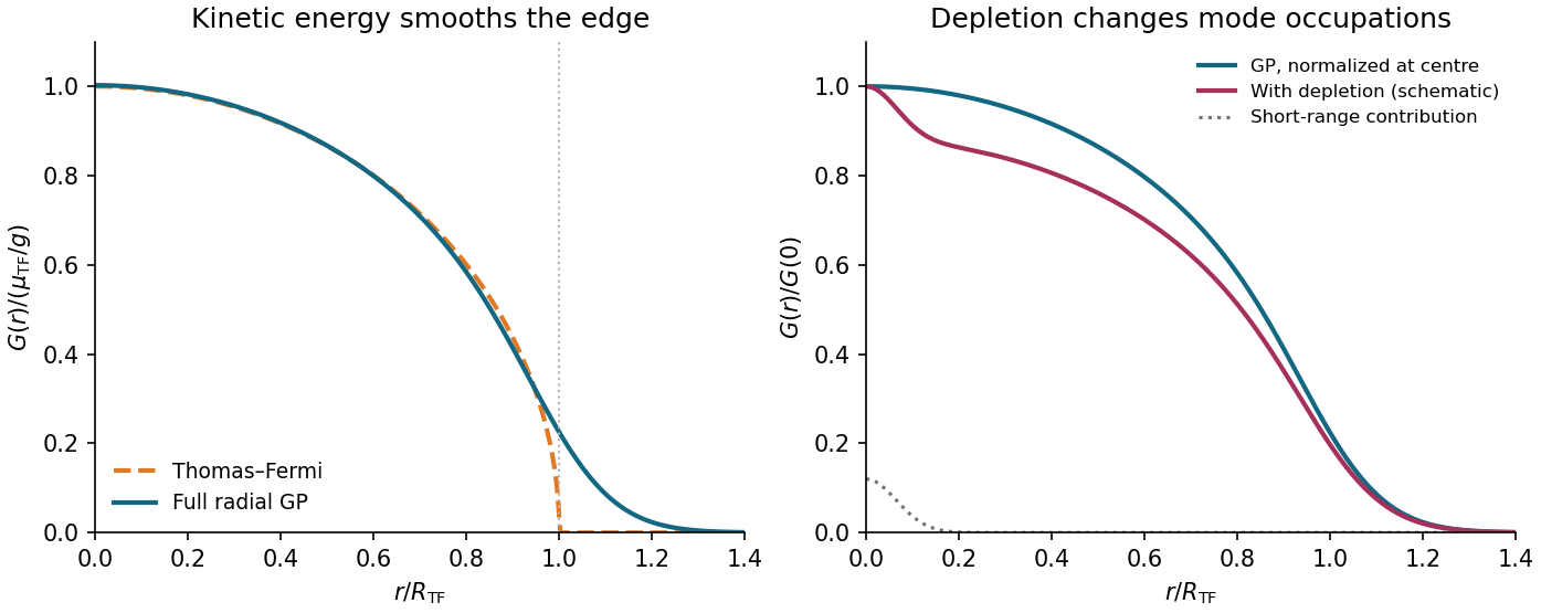
The approximation is best at the centre, $r=0$, and worst near the edge, $r=R$. For example its omitted quantum pressure of a condensate, evaluated on the interior profile, isIt is smallest at the centre and diverges at the artificial sharp edge. The central healing length ${\xi }_0=\hslash /\sqrt{2m\mu }$ is much smaller than $R$ when $\mu \gg \hslash \omega$, since $R/{\xi }_0=2\mu /(\hslash \omega )$. This is the bulk validity condition; the full Gross–Pitaevskii equation smooths the edge and gives a decaying tail outside $R$.

The Hartree product state underlying the Gross–Pitaevskii equation has the factorized one-body coherence of a Hartree condensate. Choosing its nodeless ground state orbital real givesIn particular, the Thomas–Fermi approximation for a condensate from part (d) predictsThe curve starts at $\mu /g$, decreases with zero slope at the origin, and reaches zero with an infinite slope at $R$. Restoring the kinetic energy in the full Gross–Pitaevskii equation rounds that edge and produces a nonzero tail. This corrects the Thomas–Fermi approximation for a condensate, but the resulting one-body density matrix still factorizes.

The additional missing physics is quantum depletion. Interactions scatter pairs of bosons into orbitals outside the Bose-Einstein condensate even at zero temperature. In terms of the true Bose-Einstein condensate orbital ${\phi }_0$ the exact one-body density matrix decomposes asThe single-orbital Hartree product state sets $N_0=N$ and omits ${\rho }_{\mathrm{ex}}$ altogether. In a weakly interacting Bose gas, Bogoliubov theory adds a comparatively short-range noncondensed contribution near the origin, together with reduced weight in the broad Bose-Einstein condensate component. The central value remains the total number density, not just the condensate density. Its numerical shift relative to the original Gross–Pitaevskii equation solution also depends on the interaction-induced redistribution of number density; it is not fixed by the condensate fraction alone.