Past exam of the soft condensed matter course of the University of Cambridge / 2012 / Paper 1 / 4

In linear viscoelasticity, stress is a linear functional of past strain increments: scaling the deformation scales the response, and responses to small deformations add. For a time-translation-invariant material, Boltzmann superposition writes $\sigma (t)={\int }_{-\infty }^{t}G(t-s)\dot{ϵ}(s)ds$, where $G$ is a relaxation modulus. The material combines reversible storage with delayed or dissipative response; the description is restricted to small deformations about the chosen state.

The Maxwell model places an elastic spring and viscous dashpot in series. They carry the same shear stress $\sigma$, and their shear strains add:Differentiating givesHere $ϵ$ is dimensionless shear strain, $\sigma$ shear stress in pascals, $G_0$ the spring shear modulus, $\eta$ dashpot viscosity in $\mathrm{Pa}\mathrm{s}$, and $\tau$ the relaxation time. The first term describes changing elastic strain; the second is viscous flow. In this model the material flows at long times and has zero static shear modulus.

A relaxation modulus is measured by imposing a step of strain and then holding that strain fixed. Let its amplitude be ${ϵ}_0$, so the initial stress jump is ${\sigma }_0=G_0{ϵ}_0$. For $t>0$, $\dot{ϵ}=0$ and the Maxwell model givesThe initial stress in the wording must be understood as that produced by the initial deformation. If an external apparatus instead maintains $\sigma ={\sigma }_0$, the stress does not decay: the experiment is creep, considered below. Merely specifying an initial stress without a subsequent constraint would not uniquely prescribe the relaxation experiment.

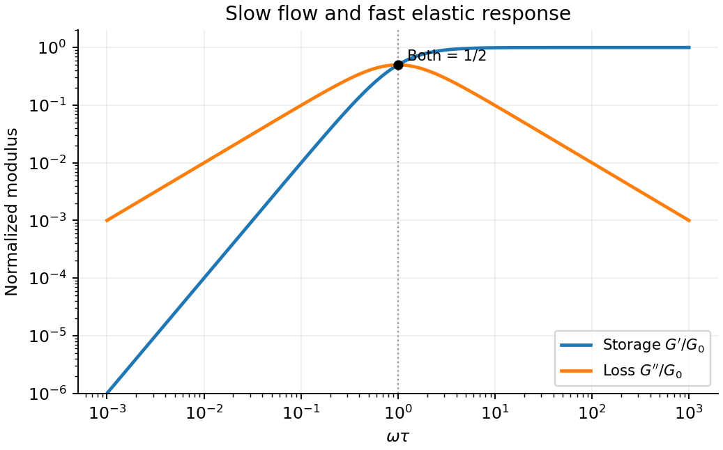
Choose complex amplitudes proportional to $e^{i\omega t}$ and define $\tilde{\sigma }=G^{\ast }(\omega )\widetilde{ϵ}$. The Maxwell model givesRationalizing the denominator yields the storage modulus and loss modulus:For $\omega \tau \ll 1$, $G^{\prime \prime }\simeq \eta \omega$ dominates and $G^{\prime }\simeq G_0{\omega }^2{\tau }^2$ is small: the material has time to flow. For $\omega \tau \gg 1$, $G^{\prime }\to G_0$ and $G^{\prime \prime }\simeq G_0/(\omega \tau )$: the dashpot scarcely deforms during a cycle and the response is mainly elastic. At $\omega \tau =1$, $G^{\prime }=G^{\prime \prime }=G_0/2$, and $G^{\prime \prime }$ is maximal. The stress leads strain by $\delta =\arctan (G^{\prime \prime }/G^{\prime })$, ranging from nearly $\pi /2$ to nearly zero.

For a fixed strain amplitude ${ϵ}_a$, dissipation per cycle is $\pi G^{\prime \prime }{ϵ}_a^2$. A peak in $G^{\prime \prime }$ therefore concerns that normalization. At fixed stress amplitude ${\sigma }_a$, it is instead $\pi {\sigma }_a^2/(\eta \omega )$, so it has no finite-frequency maximum in this ideal model. Reversing the Fourier time convention reverses the imaginary-part sign, while the physical dissipated energy remains positive.

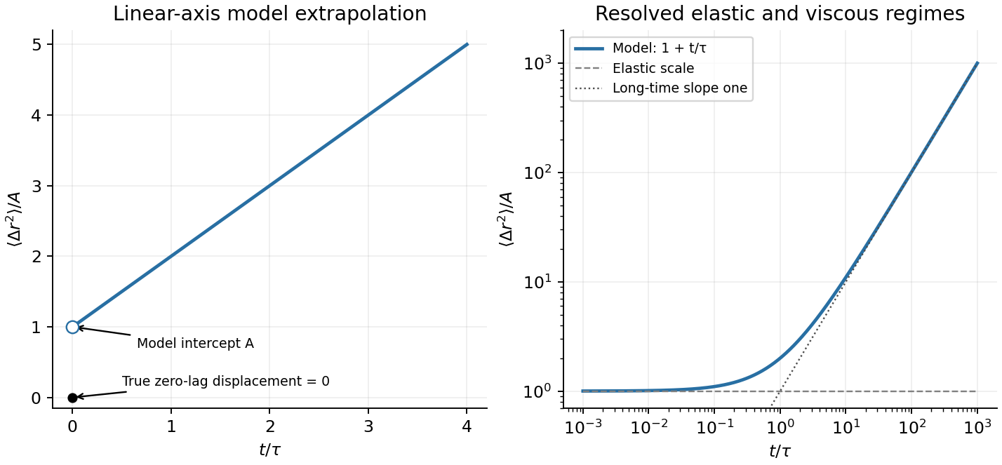
A creep experiment applies a small step of stress and holds it constant while recording strain. For $\sigma ={\sigma }_{0}H(t)$, the series spring jumps by ${\sigma }_0/G_0$ and the dashpot subsequently flows at constant rate ${\sigma }_0/\eta$. The creep compliance is thusUsing the stipulated effective stress and strain substitutions givesOn linear axes the model is a straight line of positive intercept $A=k_{B}T/(\pi a{G}_0)$ and slope $A/\tau$. On logarithmic axes it has an approximate elastic plateau for $t\ll \tau$ and slope one for $t\gg \tau$, within the time window where the continuum approximation applies. The long-time slope is $6D$ with $D=k_{B}T/(6\pi \eta a)$, agreeing with the Stokes–Einstein relation.

There is an essential zero-lag convention. A literal lag displacement $\Delta \mathbf{r}(t)=\mathbf{r}(t_0+t)-\mathbf{r}(t_0)$ has $⟨|\Delta \mathbf{r}(0){|}^2⟩=0$. The nonzero intercept above is the spring-compliance extrapolation of the idealized microrheology of a Maxwell fluid, after unresolved solvent or inertial transients. It must not be interpreted as an instantaneous finite physical displacement at exactly zero lag. The stated mesh condition motivates a continuum probe response; quantitative use is more reliable for $a\gg m$ than merely $a>m$.

For a thermally elastic network, estimate one elastically active element per mesh volume. Each contributes an elastic free-energy scale of order $k_{B}T$, giving the entropic network modulusat $T=298\mathrm{K}$. Mesh size alone would not determine the modulus of an arbitrary bending-dominated or athermal network; this is the entropic scaling assumption needed for the estimate.

The formal elastic intercept in the given model is consequentlyThe corresponding three-dimensional root-mean-square displacement is about $0.20\mu \mathrm{m}$. The temperature cancels from this estimate because the assumed modulus is itself proportional to $T$. This is the extrapolated plateau from the preceding part, not a nonzero exact zero-lag displacement. Here $m/a=1/2$, so a continuum estimate is only approximate.

In passive microrheology, track dilute inert probe spheres by video microscopy and average squared lag displacements over starting times and probes. An isotropic two-dimensional image gives $⟨\Delta r^2{⟩}_{3d}=(3/2)⟨\Delta r^2{⟩}_{2d}$. Alternatively, dynamic light scattering probes ensemble displacement statistics; the original optical microrheology study compared inferred storage and loss moduli with mechanical measurements.^[ref]

Remove drift, calibrate spatial scale and frame timing, estimate localization noise using an immobilized-bead control, and account for motion blur. Keep probes away from walls and check that changing probe radius or tracer concentration does not change the inferred bulk response unexpectedly. Noise alone can generate a false short-time intercept, while adsorption or confinement can mimic elasticity. No numerical long-time slope is fixed because a numerical viscosity is not supplied.