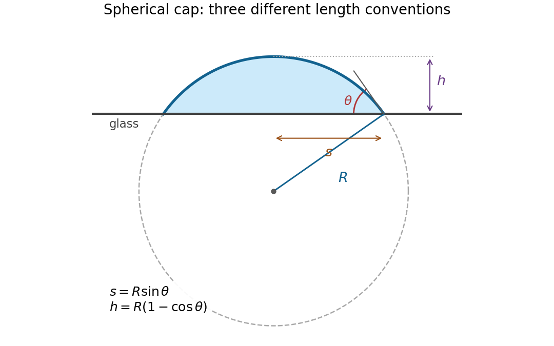
The relevant comparison is between gravity and surface tension. With the mass density difference , the Bond number and capillary length areThus the drop is small compared with the capillary length; hydrostatic pressure variations only weakly perturb its shape. The Young–Laplace equation then gives approximately constant interfacial mean curvature, and an axisymmetric drop on a uniform flat substrate is a spherical cap. The substrate selects the contact angle, measured through the water.
Write for the radius of the generating sphere, for the contact-circle radius, and for the apex height. Elementary trigonometric identities giveTaking the stated droplet radius to mean its radius of curvature, , givesThere is no diagram or explicit radius convention in the original PDF. If instead denotes the contact-circle radius, the answer is . If it denotes the radius of an equal-volume free sphere, use the volume of a spherical cap, , to obtain . The spherical cap approximation is justified in all three conventions; a unique numerical height requires specifying which radius is meant.

By definition, the relaxation modulus is the stress generated by a unit step of strain from an initially relaxed state. Set , where is the Heaviside step function, and write . Integrating the linear ordinary differential equation across the step shows that neither nor can jump: a jump would produce a Dirac delta function or its derivative, absent from the forcing. Hence .
For , a particular solution is . The characteristic equation factors asso . The initial conditions give and , whenceThe time and modulus units are those implicit in the printed coefficients. A Laplace transform check gives .
The original PDF really does put undifferentiated strain on the right-hand side. The resulting response rises from zero to one, with , rather than exhibiting ordinary stress relaxation. There is a stronger physical problem if this is intended as a passive material law: with the convention the stress-to-strain amplitude ratio isThe loss modulus would give negative cycle-averaged supplied power , contrary to passivity in linear viscoelasticity. The boxed expression is therefore the formal relaxation modulus of the equation as printed, not a claim that this equation describes an ordinary passive viscoelasticity model. No derivative of the input has been silently inserted.
Treat the liposome using the usual incompressible-tail packing model of a lipid bilayer: neglect the head-group thickness and let be the volume filling the hydrophobic part of the lipid vesicle. Both membrane leaflets have area per head group. Put , and let be the unknown outer radius. Counting molecules from the inner and outer surface areas givesEquating the total molecular volume to the volume of the spherical shell therefore givesTo prove uniqueness in the physical domain , defineIts derivative isAlso and as . By continuity and strict monotonicity, has exactly one solution with . This proves the required uniqueness without choosing among ambiguous branches of a cubic formula.
The maximum tail length is a physical admissibility bound, not automatically the actual leaflet thickness. If is the radius where the two tail regions meet, separate membrane leaflet volume balances giveThe unique candidate must satisfyIn particular is necessary. The premise that a lipid vesicle has assembled supplies this compatibility: arbitrary positive choices of need not allow any such lipid bilayer. For a very large vesicle the two thicknesses tend to , so . Setting the thickness equal to for every molecule would confuse maximum extension with actual packing. The volume-balance argument and its domain are an example of uniqueness of the packed spherical bilayer radius.
For an ideal chain, independent Kuhn length steps give the random walk relationwhere denotes the end-to-end displacement of a subchain. Equivalently the mass-size fractal exponent is . Numerical factors depend on the chosen definition of blob diameter.
A subchain smaller than the adsorption height explores three dimensions much as a free ideal chain does. At scales exceeding , adsorption restricts its perpendicular extent to order , so the coil is anisotropic. Its in-plane projection may still have a random walk law for an ideal chain, but the isotropic three-dimensional blob construction cannot be extrapolated to . This is the reason to use adsorption blobs of size .
Here is the absolute temperature and the Boltzmann constant. An adsorption blob contains monomers, so there are such blobs. Confining a blob removes an amount of conformational entropy of order ; thus the positive confinement contribution to the Helmholtz free energy isThe statement about one blob's entropy is used as an entropy loss relative to the free chain, rather than as an absolute entropy.
In the assumed slab model, contacts occur within a monomer-scale distance of the substrate. The contact fraction is approximately , giving . Multiplying this by the negative contact energy yieldsThe two contributions express the competition between loss of conformational entropy and gain of adsorption energy. The numerical coefficients are the ones stipulated by this blob approximation.
Minimize the Helmholtz free energy at fixed . Its derivative isThe physical stationary point for isTo check the minimum directly, put . Then , which is globally minimized at . The binding free energy gain per monomer is consequently .
The weak-adsorption blob picture requires , or in this model. If is too large, the layer saturates at a monomer-scale thickness; if too small, a many-blob adsorbed layer has not formed.
The stretched segment is a Gaussian chain of Kuhn length steps, with unperturbed root-mean-square end-to-end distance . Its end-to-end probability density is proportional to , so its leading elastic Helmholtz free energy is . Adding the remaining segment's adsorption free energy givesAn additive constant independent of is irrelevant. At the optimal adsorption height this becomesThe original PDF's hint labels the positive quantity proportional to an entropy. It has units of energy and is the stretching free energy. The corresponding change of conformational entropy is . This dimensional and sign correction is essential to the minimization.
This is the leading extensive Gaussian chain approximation: endpoint normalization and junction corrections give subleading terms. It requires many stretched monomers and , rather than extension near the full contour length.
During slow peeling in atomic force microscopy, adjusts to minimize the Helmholtz free energy at each imposed height. Define the positive binding gain for the adsorbed segment. The stationary point satisfiesSince , this is a minimum while . The upward pulling force is the height derivative of the minimized free energy. The implicit term vanishes because , givingUsing ,It is independent of : extra pulling height releases more monomers while leaving the fractional extension of the stretched part unchanged. Equivalently . This is the equilibrium peeling force of an adsorbed Gaussian chain.
The plateau ends when , atThereafter all monomers are detached and the Gaussian chain force is , agreeing continuously with the plateau at . Very near the start and final release, finite-chain and junction effects lie outside the blob approximation.
For the usual interpretation of a real chain in a good solvent, the detachment force is smaller in the weak-adsorption regime. Excluded volume swells the chain, increasing the cost of confinement near the substrate. The adsorbed layer becomes thicker and its binding free energy per monomer decreases. The same contact energy therefore does not mean the same total binding strength.
The scaling argument can include both adsorption and stretching. Let , where for an ideal chain and approximately for a self-avoiding walk in three dimensions. With the same contact-fraction approximation,Minimization gives and . At detachment, a tensile blob of size costs approximately ; its monomer count is . Equating the stretching gain per monomer to givesThus , compared with , so their ratio scales as for weak attraction. These are scaling relations, not exact prefactors. The real-chain adsorption exponents here use the same simple uniform-contact model as the earlier parts; a more detailed surface theory of critical phenomena can refine them. The thicker, more weakly bound layer reflects the higher cost of confining a good solvent chain.[ref]
https://dasher.wustl.edu/bio5357/readings/rubinstein-chapter3.pdf. Rubinstein and Colby, Polymer Physics, chapter 3, equations (3.59)–(3.66)
“Real” alone does not specify solvent quality: a collapsed chain in a poor solvent, strong adsorption, or substantial bending stiffness requires a different comparison. The smaller-force conclusion concerns the flexible good solvent chain implicit in the excluded-volume correction.
The gap is not a fixed mechanical separation. Thermal fluctuations of the wall compete with drift towards the microtubule under the opposing force. A monomer can be incorporated only after the gap reaches its length. The Smoluchowski equation describes this overdamped drift and diffusion of gap probability density.
For gap potential energy , the equation and its probability current areThe drift mobility is , the overdamped consequence of the fluctuation-dissipation relation for a Langevin particle. Equivalently, this coefficient is fixed by requiring the zero-current solution to be the Boltzmann distribution . Solve this equation with the appropriate exclusion, incorporation and probability-normalization conditions. The steady flux through the incorporation threshold gives the addition rate ; the elongation speed is .
There is a regime distinction in the printed problem. The absorbing boundary imposed in part (c) means instantaneous incorporation once a gap opens, and leads to the diffusion-limited Brownian ratchet with constant load. A genuinely reaction-limited polymerization Brownian ratchet instead assumes fast gap equilibration followed by a finite chemical addition rate, giving an exponential gating factor multiplying that chemical rate. The equations requested in the subsequent parts specify the former model, which is the one solved here.
In the steady state, conservation of probability requires , so is constant. The sign is positive because increasing gap reaches the incorporation boundary, whereas the deterministic drift points towards smaller gap. ThusAn integrating factor givesSubstitution makes the check particularly transparent:so . The constant offset is necessary for nonzero transport; a pure Boltzmann distribution would have and could not describe a steady succession of addition events. The limit is taken after applying the boundary conditions, avoiding the apparent singularity of the displayed parametrization.
In this polymerization Brownian ratchet model, a gap of width immediately accommodates one monomer. That event advances the tip by and resets the gap to zero. The threshold is therefore an absorbing boundary condition for a diffusion,All waiting-time probability lies within , so the steady occupation probability density satisfiesThere is a reinjection flux at equal to the absorption flux at . The nonpenetration constraint at zero is a reflecting boundary condition for a diffusion during each individual waiting episode. For the stationary reset process it must not be confused with setting the net current to zero: the source at reset supplies . This is how a normalized steady density can coexist with a nonzero exit flux.
Put and . The absorbing boundary condition for a diffusion gives , henceThis is nonnegative throughout the allowed interval. Normalizing the probability density givesThereforeEquivalently the normalized density isThe denominator is positive for , since . The dimensions are consistent: has units of inverse time, and of inverse length, and is dimensionless.
For a small opposing force, the relevant parameter is . A Taylor series givessoIn particular the zero-force rate is finite, despite the numerator and denominator of the original expression both vanishing.
For , the exponential dominates the denominator:Opening a monomer-sized gap is exponentially rare at high opposing force. The algebraic prefactor belongs to this first-passage model and must not be discarded when quoting the leading asymptotic rate.
Each addition starts a new statistically identical waiting episode at zero gap. Thus the addition rate is the reciprocal of a mean first-passage time, not the reciprocal of the mean gap:This can also be derived without the steady density. If is the mean time to reach starting at gap , its backward Smoluchowski equation isThe first boundary is reflecting and the second absorbing. An integrating factor gives , whenceAt weak force, is the time for a freely diffusing wall to move a monomer length, with reflection at the tip. At strong force, opening the gap requires work , with Boltzmann distribution suppression . The drift establishes a near-tip thermal length and a diffusion time ; consequentlyThe exponentially long wait explains why the growth slows. There is no additional chemical waiting time in the imposed absorbing-threshold model; such a time would be needed to describe the separate reaction-limited polymerization Brownian ratchet regime.
In a magnesium chloride chemical solution, the principal pair interactions are hard sphere exclusion, repulsion of overlapping electric double layers, and attractive Van der Waals forces. The positive surface attracts chloride counterions and repels magnesium coions; mobile ions screen the bare Coulomb's law interaction. The competition between screened electrostatic repulsion and Van der Waals force attraction is described by DLVO theory.
For well-separated identical weakly charged spheres, the approximate repulsive pair potential energy, at centre separation , isIt is a screened Coulomb pair potential. An attractive Hamaker constant adds a negative short-range contribution, while overlap is forbidden. Very near contact, solvation and molecular surface structure can also matter. No polymer-induced interaction should be assumed before polymer is added in part (f).
The particle carries positive surface charge density . Its surrounding electric double layer has an excess of negative chloride counterions and a deficit of positive magnesium coions. Thus decreases to zero, decreases towards its bulk value, and increases towards its bulk value. The diffuse charge density is negative and tends to zero.
If denotes the bulk number of dissolved salt formula units per unit volume, the far-field number densities are and . The bulk is neutral even though these number densities differ. In the dilute mean-field picture the total diffuse electric charge is , ensuring overall electroneutrality. A molecularly bound compact layer would require additional surface-chemistry information and is not assumed in the supplied potential.
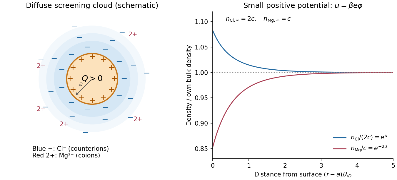

Let be the permittivity, , the elementary charge, and the bulk salt formula-unit number density. The Boltzmann distribution givesConsequently the exterior Poisson-Boltzmann equation isFor small , meaning , linearize the exponentials. The Debye–Hückel approximation givesThis is also : the divalent cation contributes and the two monovalent anions contribute . In terms of molar salt concentration in , replace by ; if is in , use . The molar ionic strength is in the same concentration units.
The boundary conditions are and, by Gauss's law,Here the surface charge is uniform and the spherically symmetric interior field is zero. Set ; the radial equation reduces to . Decay excludes the growing exponential, so write . Then , givingIt solves the linearized Poisson-Boltzmann equation, not the full nonlinear equation at finite . The radial ion profiles, consistently to first order, areThe exponential Boltzmann distribution formulas above express the full mean-field relation, but substituting a linearized potential into them is accurate only to the retained order. A useful electroneutrality check isThe result is the Debye-Hückel potential of a charged sphere.
Write the particle volume fraction as . In a stable, repulsion-dominated colloid, low gives a disordered fluid. Increasing makes the interaction between neighboring particles important and can produce an ordered crystal, separated from the fluid by a phase coexistence curve. Increasing the Debye–Hückel screening length at fixed charge strengthens the repulsion at a given separation and allows freezing at smaller geometrical volume fraction.
The geometric intuition is that particles behave as though they occupy more than their bare diameter: roughly, an effective exclusion diameter extends out to the separation where is of order . A hard sphere comparison then uses . This explains the trend; it is not an exact freezing criterion.
At short Debye–Hückel screening length and negligible attraction, the diagram approaches hard sphere fluid–crystal coexistence. For longer-ranged soft repulsion, body-centered cubic lattice and face-centered cubic lattice crystals can both be stable, with the former often appearing towards the softer, lower-density freezing boundary. Screened-Coulomb simulations exhibit both these crystal structures.[ref]
https://doi.org/10.1103/PhysRevLett.57.2694. Kremer, Robbins and Grest, Phase Diagram of Yukawa Systems: Model for Charge-Stabilized Colloids
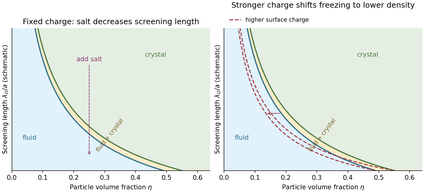

No universal quantitative diagram follows from alone: the charge, Hamaker constant and surface conditions must also be fixed. If salt suppresses the stabilizing barrier enough for Van der Waals force attraction to dominate, a colloid-poor/colloid-rich separation or aggregation can replace part of this repulsive reference diagram. Dense colloidal glasses or colloidal gels may also be observed after kinetic arrest; they should not be mistaken for additional thermodynamic equilibrium thermodynamic phases.
First hold the surface electric charge fixed and increase the bulk salt concentration. Since , the Debye–Hückel screening length decreases as . For surface gap ,Thus both the range and the strength of repulsion decrease. In the repulsive phase diagram, the sample moves downwards at fixed volume fraction and can melt from a crystal into a fluid. Because screening length is already a diagram axis, changing salt moves the state through that diagram rather than independently changing its fixed-charge coexistence curves. If Van der Waals forces become dominant, however, adding salt may instead destabilize the dispersion and cause aggregation. These are distinct physical regimes.
Second increase at fixed salt concentration and particle size. The electric charge is , so the pair repulsion increases approximately as within the Debye–Hückel approximation, while the reservoir screening length remains unchanged. Freezing then becomes possible at lower volume fraction or shorter screening length. At fixed , the coexistence curves shift towards lower ; a previously fluid sample may crystallize.
These statements assume fixed, uniform charge and a salt reservoir dominating the screening. Strong charging requires nonlinear screening and possibly charge regulation. At very low added salt or appreciable particle concentration, particle-released counterions also contribute to ionic strength, so the screening length is no longer independently fixed by the added salt alone.
For dissolved, nonadsorbing polyethylene glycol, the usual new interaction is a depletion force. Polymer centres are excluded from a layer of thickness of order their radius of gyration around each particle. When the particles approach, their exclusion layers overlap. This increases the volume accessible to polymer and its translational entropy, lowering the colloid pair free energy. Equivalently the surrounding polymer osmotic pressure pushes the particles together.
In the dilute-polymer Asakura-Oosawa model, let be the surface gap and . Thenfor , and for . Here is the reservoir polymer osmotic pressure. The overlap-volume formula follows by adding two equal spherical cap volumes with height . Thus the added attraction has range about and grows with polymer concentration. The total interaction is approximately hard exclusion plus screened electrostatic repulsion plus Van der Waals force and depletion attractions.
Increasing polymer concentration therefore creates a family of phase diagrams, rather than a unique shift determined by polymer size alone. Where the attraction overcomes repulsion, colloid-poor fluid can coexist with a colloid-rich phase, and fluid–crystal coexistence generally broadens. For sufficiently long-ranged attraction, stable fluid–fluid separation can occur. For the stipulated small polymer, the attraction is short-ranged: fluid–fluid separation can be metastable to crystallization, and a rapid attraction increase can instead produce an arrested colloidal gel. Residual long-ranged repulsion can oppose bulk separation. Simulations and free-volume calculations confirm that longer-ranged electrostatic repulsion can counteract depletion-driven separation.[ref]
https://arxiv.org/abs/cond-mat/0509790. Fortini, Dijkstra and Tuinier, Phase behaviour of charged colloidal sphere dispersions with added polymer chains
The nonadsorption assumption matters. If the polyethylene glycol adsorbs to the particles, a dense attached layer can give steric stabilization, whereas chains attaching to two particles can produce polymer bridging. The paper does not specify surface affinity or polymer concentration, so depletion is the standard conditional answer, not a prediction of an inevitable particular final phase.
In the weak-field reptation regime of agarose gel electrophoresis, the electrophoretic mobility of a long linear DNA chain scales as , where is its number of base pairs. One way to see the scaling is that the constrained-chain diffusion coefficient scales as , whereas its effective electric charge scales as ; the drift response is proportional to . With the same electric field and running time, the migration distance is therefore . The time cancels from the ratio, givingHere “kbp” means a thousand base pairs, not a rate. The second gel band has traveled farther and corresponds to the shorter chain under this migration model. The inverse-length law applies only over an appropriate migration regime.[ref].
At very low agarose concentration the mesh becomes too open to sieve these chains effectively. In the free-solution limit the chain's electric charge and friction are both approximately proportional to its length, so both chains have nearly the same electrophoretic mobility and their gel bands cease to separate well. At very high agarose concentration the pores become small and transport is strongly hindered; over a fixed experimental time both chains migrate very little, so their absolute spatial separation again becomes small. Increasing gel concentration can improve resolution over an intermediate range, but not indefinitely.
The numerical result is conditional on the inverse-length reptation law. Actual gel electrophoresis size calibration often uses an empirical approximately linear relation between distance and over a specified range. One known band alone cannot fix that relation's slope. The PDF supplies neither gel concentration nor a calibration curve, so is the standard model estimate rather than a uniquely calibrated experimental size.
Choose a coordinate measured from the sphere centre towards increasing distance from the block, so an atom in the sphere is at height . Summing the atom–block potential energy with the sphere's number density givesFor , a uniformly valid Taylor series over the sphere isThe odd moments vanish by reflection symmetry. The sphere volume is , and its second moment isConsequentlyThe first finite-radius correction is therefore . There is no relative correction because the first moment about the centre is zero. The leading term is just the number of sphere atoms times the potential at its centre; the correction increases the attraction because the nearer atoms contribute more strongly than the farther atoms lose.
This is the far-field sphere-plane dispersion energy, with Hamaker constant . It must be distinguished from the near-contact sphere-plane dispersion force, whose small parameter is the surface gap divided by the radius. Here is explicitly the centre-to-plane distance.
Let increase down the pipe, be its radius and the distance from its axis. For steady, fully developed laminar flow of a Newtonian fluid, the axial Navier-Stokes equations reduce toWrite . Integrating twice, regularity at excludes a logarithmic term, and the no-slip boundary condition gives the Hagen-Poiseuille flow profileThe volumetric flow rate follows by integrating over the circular cross-section:For the intended gravity-driven case with no imposed axial pressure gradient, . Substitution givesandThe corresponding mean speed is about and the diameter-based Reynolds number is , consistent with laminar flow. The original PDF does not specify inlet and outlet pressures. If they impose an additional pressure gradient, the general result with above applies; gravity alone does not determine that extra contribution.
Use a rheometer, for example a cone-and-plate rheometer or a parallel-plate rheometer, to impose a small deformation and measure the required torque, or impose a torque and measure the deformation. The apparatus geometry converts these into shear stress and strain. First check that reducing the imposed amplitude does not change the normalized response; this identifies the linear regime and avoids yielding or structural rearrangement.
Three complementary protocols characterize the material's memory. In a stress relaxation experiment impose a small step and hold the deformation fixed. The output is the relaxation modulus , revealing how stored stress decays and whether an elastic plateau remains. In a creep compliance measurement impose a small stress step and record . Removing the load also distinguishes recoverable deformation from permanent flow.
In small-amplitude oscillatory shear, impose sinusoidal strain over a range of frequencies and measure both stress amplitude and phase. With , fitThe outputs are the storage modulus and loss modulus , or equivalently amplitude ratio and loss tangent . These measure elastic storage and dissipative response, respectively. The step experiments give time-domain information and the oscillatory experiment gives the corresponding frequency-domain response. All comparisons must use the same deformation convention and controlled temperature.
The dynamic modulus, or complex viscoelastic modulus, is the ratio of complex stress amplitude to complex strain amplitude in the periodic steady response:This defines the sign convention; for passive response the loss modulus is nonnegative at positive frequency. A Newtonian fluid obeys , while a Hooke's law solid obeys . HenceThe first is purely dissipative and the second purely elastic. Here denotes the scalar deformation used in the problem, with any shear-versus-extension geometric factors already included in its modulus and viscosity.
Parallel elements have the same strain, while their stresses add. The spring supplies and the viscous element supplies , so the Kelvin-Voigt model has constitutive equationFor the oscillatory deformation this givesPhysical stress and strain are the real parts of these expressions. Thus the storage modulus is , independent of frequency, and the loss modulus is . The equation is the quasistatic material law; an inertial equation for an attached mass would require additional mechanical data.
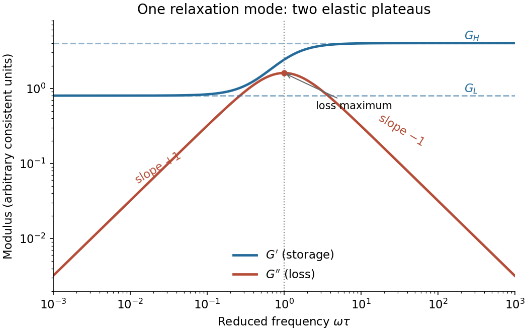
For elements in series the stress is common and the strains add. If and are the Kelvin element and added spring amplitudes, thenThe compliances therefore add, yieldingThis is a standard linear solid model. DefineWriting , its storage modulus and loss modulus areThus increases from the low-frequency plateau to the high-frequency plateau . The loss modulus has low-frequency slope and high-frequency slope on a log-log plot, with maximum at . At that frequency . There need not be a crossing of the two curves for arbitrary spring constants.

A Kelvin-Voigt model has no finite instantaneous elastic compliance: the viscous element prevents a sudden deformation under a finite stress step. Its creep compliance isConversely an ideal strain step requires an impulsive stress,After the impulse the held-strain response is simply constant. There is no finite stress-decay interval, and the loss modulus grows without bound as . This fails to represent a material with both a finite instantaneous stiffness and delayed stress relaxation.
The added series spring resolves this particular defect. At the instant of loading the Kelvin element cannot move but the added spring can. The standard linear solid model consequently hasandIts instantaneous stiffness is , its long-time stiffness is , and it exhibits genuine stress relaxation as well as delayed creep. The creep retardation time differs from the stress-relaxation time . These properties also follow directly from its constitutive equation,It remains an idealized solid with one relaxation mode: it cannot describe unrestricted long-time viscous flow, nonlinear response, or a broad spectrum of relaxation times.
A hydrophobic surface is poorly wetted by water: on a smooth surface its equilibrium contact angle, measured through the liquid, exceeds . A drop therefore tends to bead up, limiting its contact area. Hydrophobicity does not mean that the surface exerts a mysterious repulsive force on every water molecule.
The waxy coating has a largely nonpolar exterior. Water molecules form favorable hydrogen bonds with one another, whereas a hydrocarbon-rich wax surface offers few suitable hydrogen bond donors or hydrogen bond acceptors. Water–surface adhesion is weak relative to water's cohesion. The drop shape minimizes the combined solid–air, solid–water and water–air interfacial free energies, not merely the liquid's exposed area.
In terms of Young's equation, . A contact angle greater than corresponds to : replacing dry surface by wetted surface has an interfacial cost. The balancing liquid interface then favors a small wetted patch. Microscopic leaf texture can amplify the apparent hydrophobicity, especially when it traps air under the drop as a Cassie–Baxter state; the chemistry of a smooth wax layer alone does not guarantee an extremely large apparent angle.
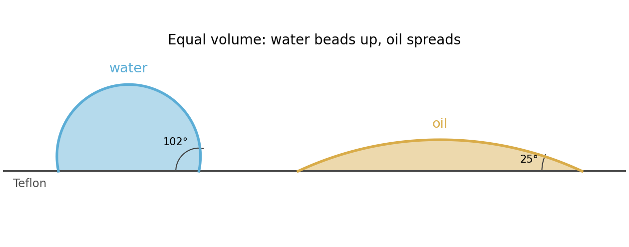
On Teflon, the water drop has an obtuse contact angle and beads up, whereas the oil drop has an acute contact angle and spreads into a shallower patch. For small drops with negligible Bond number, both can be drawn as spherical caps.
To compare shape at equal volume , let denote the generating sphere radius. The cap height and footprint radius areFor a fixed , these relations give a taller, narrower drop for the larger contact angle. The angles are measured inside the liquid, including the obtuse angle of the water drop.

For an ideal smooth homogeneous substrate in thermodynamic equilibrium, Young's equation iswhere denotes air, the solid, and the chosen liquid. It follows either by balancing tangential interfacial forces at the contact line or by varying the wetted area at fixed drop volume.
The dry Teflon–air surface energy is the same in the two measurements, so subtracting the two equations eliminates it:ThereforeThe water–Teflon interface has the higher interfacial free energy per unit area. Neither individual solid–liquid surface energy is determined without the solid–air value; the difference is determined.
Colloidal particles experience attractive Van der Waals forces, arising from correlated molecular charge fluctuations and other dipolar interactions. Integrating many weak molecular attractions over two particles can give a deep near-contact well. For identical spheres of radius and surface gap , a positive Hamaker constant gives approximatelyBrownian motion brings particles into encounters. Without a repulsive barrier, they can reach the attractive primary minimum; if the binding energy is much larger than , thermal motion rarely separates them again. Repeated sticking produces aggregates. This is a kinetic stability statement: thermal agitation causes encounters but does not itself supply a stabilizing interparticle repulsion. The molecular cutoff and hard sphere exclusion prevent the unphysical divergence of the continuum attraction.
One method is to give every particle a sufficiently large surface charge density of the same sign. For example, attach ionizable sulfonate groups covalently to the surface. Dissociation leaves negatively charged surface groups and releases mobile positive counterions into the water. A surfactant with a strongly bound head group can provide another charging route, provided it does not desorb during the experiment.
Each charged particle is surrounded by an electric double layer. As two such particles approach, overlap of these ionic clouds raises the electrostatic and ionic free energy, producing repulsion. In a dilute electrolyte, the range is set by the Debye–Hückel screening length,For identical weakly charged spheres a representative screened Coulomb pair potential isIts sum with the Van der Waals force attraction is the DLVO theory pair potential. Choose the charging level so that the repulsive barrier is many high; particles then rarely reach the primary attractive well during the observation time. This is kinetic stabilization rather than removal of all attraction.
Deionized water is useful because low added ionic strength gives a long-ranged repulsion. It does not mean that the charged dispersion contains no ions: the surface's own counterions are unavoidable and contribute to screening. Surface dissociation, contamination and particle concentration therefore matter even without added salt. An alternative valid route is a dense, firmly attached layer of water-soluble polyethylene glycol, producing steric stabilization without relying on a large electrostatic barrier.
Without stabilization, the potential energy is predominantly attractive outside the molecular core and drops into a deep primary minimum. With the charging treatment, the DLVO theory sum develops a positive barrier between distant particles and that primary minimum. The barrier must be large compared with to inhibit aggregation on the experimental timescale. A shallow secondary minimum can remain at larger separation, depending on parameters.
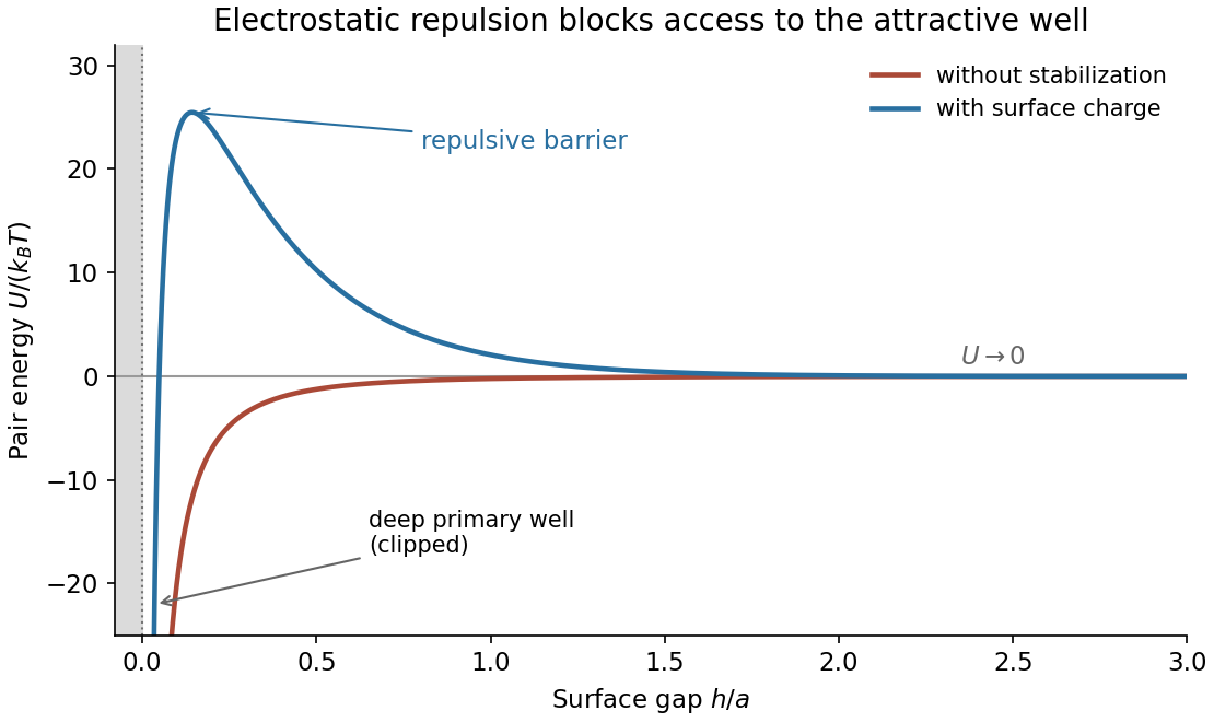
Attractive and electrostatically stabilized colloidal pair potentials
. Original illustrative curves for two equal spheres. The unstabilized curve uses the nonretarded sphere–sphere attraction; the stabilized curve adds screened electrostatic repulsion. The molecular core is excluded and the deep near-contact well is clipped by the plotting range. Potential depths and screening parameters are illustrative, not data supplied by the paper. Details.
The horizontal axis is the surface gap, so the molecular exclusion boundary is at its origin. Both interactions tend to zero at large separation. Raising salt concentration shortens the Debye–Hückel screening length and can reduce the barrier, allowing particles to stick again.
The Flory–Huggins solution theory treats a polymer solution as an incompressible lattice mixture, with one solvent molecule occupying one site and one chain occupying connected sites. Thus the supplied is naturally the mixing free energy per lattice site; if a site has volume , the free-energy density is .
The term is the polymer translational entropy of mixing contribution. There are only as many independently translating chains as monomers, which explains the factor . The term is the solvent entropy of mixing contribution. Both lower the mixing free energy for .
The term is the mean-field excess interaction contribution from replacing like contacts with polymer–solvent contacts. In the simplest energetic lattice model,where counts neighboring contacts and the are pair contact energies. Positive penalizes unlike contacts and can favor demixing. Because chain connectivity suppresses the polymer's translational mixing entropy, relatively modest unfavorable interactions can cause separation of long chains. More general effective can also include entropic effects.
Local compositional stability requires positive curvature of the mixing free energy. Differentiating twice at fixed temperature, with independent of composition as in the given model, givesThe spinodal occurs where this vanishes:Between the two spinodal compositions at sufficiently large , and a homogeneous mixture is unstable to infinitesimal composition fluctuations. The binodal is instead fixed by the common-tangent construction, and encloses a larger coexistence region. Between binodal and spinodal the mixture is locally stable but metastable.
A phase diagram with a conventional upper critical temperature additionally assumes that decreases with , for example with . Then high temperature gives a uniform mixture; cooling produces an asymmetric coexistence dome whose critical composition is on the dilute-polymer side. The spinodal lies inside the binodal dome. An arbitrary need not give this orientation, so the free-energy formula alone does not specify a unique temperature axis.

At the thermodynamic critical point, the two spinodal branches merge: and . The third derivative isFor , its zero gives . Substitution in the spinodal relation yieldsAn absolute critical temperature requires an interaction–temperature relation. Under the usual energetic approximation , define the theta temperature , at which an infinite chain has . ThenThus tends to a nonzero constant, , while . It is the temperature deficit, not itself, that scales as .
More generally, if a smooth obeys and , thenThis is the critical point of a Flory–Huggins polymer solution. The same leading chain-length exponent follows for a smooth temperature law, while its coefficient depends on the omitted solvent thermodynamics. The lattice interpretation connects the chain-length dependence of mixing entropy to the theta condition .[ref].
For , the critical polymer volume fraction isIf is the volume assigned to one amino acid in the lattice model, the critical number densities are exactlyThe extra physical approximation needed to use the given radius of gyration is that a chain in a poor solvent is a compact polymer globule. Its size then scales as with , so . This gives the standard scaling estimatesWith , numerical substitution givesUsing only the leading large- value gives and , respectively. These are scaling estimates, not geometrically exact densities.
For comparison, a specifically uniform spherical compact protein has the radius of gyration of a uniform sphere, , so its physical volume is . Taking instead gives and . The factor between these conventions is geometric. The PDF does not give a monomer volume, globule density or shape model, and a radius of gyration alone does not determine an exact molecular volume. The model-independent conclusions are the formulas in terms of and the 300:1 ratio of monomer to protein number density.
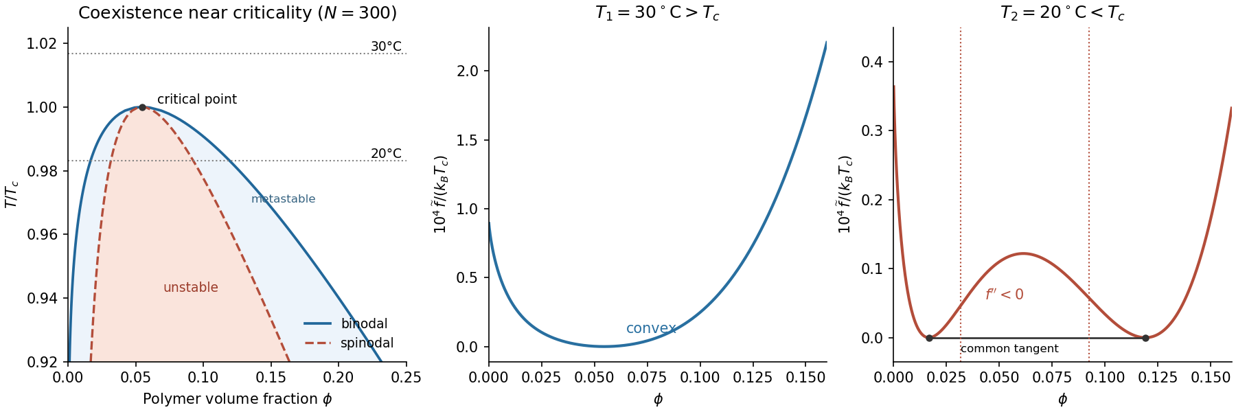
Interpret the stated transition as an upper critical miscibility temperature: cooling increases the effective through . Above , the homogeneous mixing free energy is convex throughout , with no two-phase common tangent. Below , it acquires a region with , bordered by the spinodal. A lower straight line touches the curve at two binodal compositions and ; this common-tangent construction gives the equilibrium polymer-poor and polymer-rich phases.
The precise raw curve need not have two equal minima: subtracting an affine function of changes reference chemical potentials without changing curvature or coexistence compositions. The free-energy panels above subtract the tangent at from the upper-temperature curve and the common tangent from the lower-temperature curve. This makes the common tangent and the convex-versus-nonconvex distinction visible.
If the mean initial composition lies inside the low-temperature spinodal region, an arbitrarily small separation into equal-volume regions with compositions changes the mean free energy bySmall fluctuations therefore grow spontaneously: this is spinodal decomposition. Interfacial costs limit very short-wavelength fluctuations, and the polymer-poor and polymer-rich domains subsequently coarsen towards their binodal compositions.
If lies just outside a spinodal branch but still inside the binodal, then . Small fluctuations increase free energy, so the uniform mixture is metastable. Separation requires a sufficiently large nucleus to overcome the interfacial barrier, followed by nucleation and growth. There is no guarantee that this happens rapidly. If the initial composition is outside the binodal as well, it remains a stable uniform phase after cooling.
For a mean composition in the coexistence interval, conservation of polymer fixes the volume fraction of the rich phase by the lever rule:The temperatures alone do not determine which mechanism occurs without the initial composition. Numerical free-energy curves additionally require ; the plotted example uses with absolute temperatures , and .
The Reynolds number compares inertial and viscous effects:where is fluid mass density, a characteristic swimming speed, a characteristic body length, and the dynamic viscosity. Both swimmers are in the same fluid, so the fluid properties cancel from the ratio:For an order-of-magnitude estimate, take , , and . With water values and , these giveand henceThe dimensions and swimming speeds are estimates, so this ratio is not a universal species-independent constant. Its physical significance is robust: viscous forces dominate the bacterium's motion, whereas fluid inertia is crucial for the whale.
There is a source error to resolve first. For a drag coefficient defined by , the velocity relaxation time is . The mass and drag coefficient in the PDF's exponential are interchanged: is dimensionless, whereas is not. The consistent mean relaxation law is therefore .
A mean relaxation law alone does not determine a variance. Use the usual thermal Langevin equation, with a bath at temperature and the fluctuation-dissipation relation for a Langevin particle:Here the calculation is for one component in Cartesian coordinates. With fixed initial position and velocity, integration gives the mean displacementIntegrating the stochastic part of the velocity once more gives the centered displacementThe delta correlation reduces its variance to a single integral:This is the integrated Ornstein-Uhlenbeck displacement for a prescribed initial velocity. Its short-time variance is ; at long times it is . Thus the diffusion coefficient isIf the requested mean-squared fluctuation instead refers to the conventional equilibrium mean squared displacement, the initial velocity is also averaged over its thermal distribution, with and . Its contribution adds , givingThis has the ballistic limit and the same diffusive limit . For fixed nonzero , the uncentered mean square instead equals the first boxed variance plus . In three independent spatial dimensions, the centered variances add, and the long-time result is . Stating the initial-velocity convention is necessary to distinguish these finite-time formulas.
Articles were limited to the first 100 out of 146 total.
Articles by others on the same topic
There are currently no matching articles.