Past exam of the symmetry and relativity course of the University of Oxford / 2015 (A13481W1, B2)

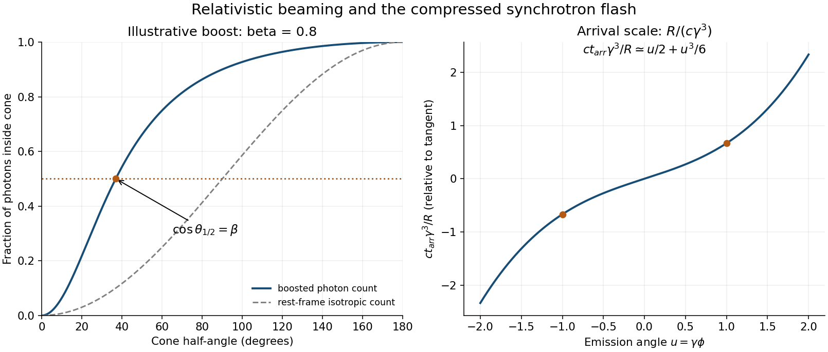
Choose the source motion along $+x$, write $\beta =v/c$, and let primes denote its instantaneous rest frame. A photon with rest-frame energy $E^{\prime }$ and direction ${\theta }^{\prime }$ has $p_x^{\prime }=E^{\prime }\cos {\theta }^{\prime }/c$ and transverse momentum $E^{\prime }\sin {\theta }^{\prime }/c$. A Lorentz boost to the laboratory givesSince $|\mathbf{p}|=E/c$, the relativistic aberration relation and its inverse areThe mapping is monotone. The boundary of the rest-frame forward hemisphere, $\cos {\theta }^{\prime }=0$, therefore maps to $\cos \theta =\beta$. An isotropic photon count assigns exactly half the photons to that hemisphere, provingThe photon count inside a relativistic beaming cone concerns an emitted ensemble and counts photons, not their total energy or the arrival-time-weighted power at a detector. The laboratory photon energies depend on direction, so “half the photons” need not mean half the radiated energy. At large $\gamma$ the angular scale is ${\theta }_{1/2}\simeq 1/\gamma$.

Use the metric $\eta =\mathrm{diag}(-1,1,1,1)$ and four-velocity $u^{\mu }=\gamma (c,\mathbf{v})$. Its derivative with respect to proper time is the four-acceleration. Sincea purely transverse laboratory acceleration has $d\gamma /dt=0$. With $d/d\tau =\gamma d/dt$,The invariant proper acceleration is the magnitude measured in the instantaneous rest frame, $a_0^2=A^{\mu }{A}_{\mu }$. Consequently,For longitudinal acceleration the factor is instead ${\gamma }^3$ multiplying the laboratory acceleration. The distinction matters for circular storage-ring motion, where the acceleration is centripetal and transverse even though its magnitude is nonzero.

Interpret $3$ GeV as the electron's total energy; the alternative kinetic-energy reading changes the estimate only slightly at this scale. The Lorentz factor and orbital acceleration areUsing the supplied Larmor formula, ${\mu }_0=1/({ϵ}_0{c}^2)$ and the revolution time $2\pi R/v$,For $R=561$ m this gives $P=1.7405\times 10^{-10}$ W per electron and $T_{\mathrm{turn}}=1.17577\times 10^{-5}$ s. Their product isThis is the energy loss of one electron on a full circular orbit, not its energy loss per metre or the total loss of the whole bunch. The fractional loss is only about $4.26\times 10^{-6}$ of the $3$ GeV energy each revolution. Maintaining a steady stored energy requires replacing that energy through the accelerator's rf system.

Relativistic relativistic aberration concentrates emission into an angular scaleThis is a half-angle or characteristic divergence scale; a full cone opening is about twice it. The exact half-photon-count cone in a applies to isotropic rest-frame emission. A synchrotron emitter has its own rest-frame angular radiation pattern, so that count result should not be treated as an exact median-power formula for the synchrotron beam. It nevertheless gives the correct relativistic beaming scale. Electron-beam emittance, vertical angular spread and the detector's acceptance can broaden the experimentally observed divergence beyond this intrinsic estimate.

A fixed distant observer receives appreciable radiation while the velocity points within an angle of order $1/\gamma$ of the line of sight. The corresponding emission interval is $\Delta t_{\mathrm{em}}\sim R/(\gamma v)$. The source moves toward the detector during that interval, shortening the light-travel distance. In the far-field limit,where $\varphi$ is the angle between velocity and the detector direction. Near the tangent, $1-\beta \cos \varphi \sim {\gamma }^{-2}$, soThe emission interval itself is of order $3.2\times 10^{-10}$ s. Omitting the arrival-time compression would therefore miss many orders of magnitude.

For a definite angular window $-1/\gamma \le \varphi \le 1/\gamma$, integrating the arrival-time relation givesThe order-one coefficient depends on how the beam window or pulse width is defined. These are intrinsic single-electron radiation-flash scales. For bunch-length broadening of synchrotron radiation, a finite bunch moving through the same tangent point contributes an arrival-time spread of order its length divided by $v$; the longitudinal bunch profile and instrumental response must be convolved with the intrinsic flash. “Short bunch” alone does not specify an experimental bunch pulse duration at the attosecond scale, because no bunch length has been supplied.^[ref]

A shorter radiation flash has a broader Fourier transform. From iii, its characteristic angular-frequency bandwidth isAt fixed bending radius this scales as ${\gamma }^3$ as $v\to c$. The standard synchrotron critical angular frequency makes the same scaling explicit:A periodically circulating electron produces harmonics of its revolution frequency. The very large harmonic range, of order ${\gamma }^3$, forms the familiar effectively continuous broad synchrotron spectrum at ordinary detector resolution. The result concerns the intrinsic spectrum of the radiation, not merely the slow envelope imposed by a long incoherent bunch. Ordinary frequency is $\nu =\omega /(2\pi )$; mixing cycles per second with radians per second would introduce a spurious factor of $2\pi$ into photon-energy estimates.^[ref]

Using the conventional critical scale rather than guessing a precise Fourier-width coefficient,This is extreme ultraviolet and the very soft X-ray boundary, with a broad spectrum extending on either side; it is not a hard, multi-keV X-ray source at the stated large bending radius. The characteristic energy is not a sharp upper cutoff. For orientation, the standard angle-integrated spectral power per unit frequency peaks near $0.29E_c\simeq 31$ eV, also in the extreme ultraviolet; a particular angular acceptance weights that spectrum differently.

The crucial scale follows from both the $3$ GeV energy and the $561$ m radius. Using only the fact that synchrotron sources can make X-rays, or replacing the bending radius by a much smaller unstated value, would misidentify the characteristic photon energies here. The critical-energy convention and the broadband character are described by the primary radiation model.^[ref]

Regard $f$ as a scalar field evaluated on a specified worldline $x^{\lambda }(\tau )$. The ordinary multivariable chain rule givesThis is the directional derivative along the four-velocity. With $x^0=ct$, it reads $df/d\tau =\gamma ({\partial }_{t}f+\mathbf{v}\cdot \nabla f)$. The spatial term is present because the worldline moves through the field; it would be lost by identifying a total derivative along the particle with a partial derivative at a fixed spatial position. For a scalar the contracted expression has the same value in all coordinate systems. For a tensor field the analogous covariant derivative also transports its indices.

Use $u^{\lambda }{u}_{\lambda }=-c^2$ and a constant Minkowski metric. Vary the velocity-dependent square root before imposing the proper-time normalization. Equivalently, vary a reparametrization-invariant worldline action first and then choose proper time. Its canonical covector momentum isThe coordinate derivative at fixed velocity is $\partial \mathcal{L}/\partial x^a=q{u}^{\lambda }{\partial }_a{A}_{\lambda }$. The Euler-Lagrange equation and the chain rule from a therefore giveDefine the antisymmetric field tensor byThe particle equation becomesAntisymmetry ensures $u^a{F}_{a\lambda }{u}^{\lambda }=0$, so the force is orthogonal to the four-velocity and preserves $u^2=-c^2$. The worldline variation before proper-time normalization is essential: substituting $\sqrt{-u^2}=c$ into the Lagrangian before taking its velocity derivative would turn the kinetic term into a constant and incorrectly remove the inertial momentum. The normalization is a property of the proper-time solution, not permission to discard the variational dependence.

For the source's definition $s^{\alpha }=\gamma (\mathbf{s}\cdot \mathbf{v}/c,\mathbf{s})$, direct contraction with $u^{\alpha }=\gamma (c,\mathbf{v})$ givesIt remains zero under the torque-free transport law. Differentiate the contraction, using the product rule and $u^2=-c^2$:Thus an initially spatial spin in the instantaneous rest frame remains orthogonal to the velocity. This is the orthogonal-spin specialization of Fermi-Walker transport. The sign is tied to the negative timelike norm; using the opposite metric sign without changing the transport formula would spoil the cancellation.

Take the dot here to mean $d/d\tau$, as in the source. Differentiate $u^{\alpha }=\gamma (c,\mathbf{v})$ and the given spin components. Their contraction simplifies because the terms involving $\dot{\gamma }$ cancel:The spatial part of the transport equation consequently readsUse $\dot{\gamma }/\gamma ={\gamma }^2\mathbf{v}\cdot \dot{\mathbf{v}}/c^2$ and divide by $\gamma$. The result isNo assumption of acceleration perpendicular to the velocity was made. In particular the second term cannot be dropped for a particle speeding up along a straight line. This $\mathbf{s}$ is the three-vector in the source's particular spin four-vector parametrization; its Euclidean magnitude need not be the invariant proper-spin magnitude.

Let the fixed direction of motion be the unit vector $\mathbf{n}$ and decompose $\mathbf{s}=s_{\parallel }\mathbf{n}+{\mathbf{s}}_{\perp }$. In ii the two parallel contributions cancel, whereas the transverse equation isFor the stated speed law, $1-v^2/c^2=e^{-2\Gamma \tau }$, hence $\gamma =e^{\Gamma \tau }$. Since the particle is initially at rest, $\gamma (0)=1$, andThe corresponding spin four-vector has components $s^0=\gamma \beta s_{\parallel }(0)$, $s_{\parallel }^{\mathrm{spatial}}=\gamma s_{\parallel }(0)$, and ${\mathbf{s}}_{\perp }^{\mathrm{spatial}}={\mathbf{s}}_{\perp }(0)$. Its squared norm is therefore $s_{\parallel }(0{)}^2+|{\mathbf{s}}_{\perp }(0){|}^2$, independent of time. The transverse decay of the source's laboratory three-vector is a boost-normalization effect, not a loss of proper angular momentum or a torque.

For a real increasing speed take $\Gamma >0$ and $\tau \ge 0$. The prescribed profile has a singular initial acceleration: $v\sim c\sqrt{2\Gamma \tau }$ near zero. The differential transport calculation applies for $\tau >0$ and the solution has the continuous initial limit displayed above. This trajectory should not be silently described as motion at constant proper acceleration.

First note that the supplied spin equation preserves $s\cdot u=0$: its electromagnetic bracket has contraction $u_a{F}^{a\lambda }{s}_{\lambda }+(u^2/c^2)F^{\mu \nu }{u}_{\mu }{s}_{\nu }=0$, and the remaining transport term cancels $s\cdot \dot{u}$ as in i.

For an explicitly electromagnetic acceleration, set ${\dot{u}}^a=(q/m)F^{a\lambda }{u}_{\lambda }$ and define $C=F^{\mu \nu }{u}_{\mu }{s}_{\nu }$. Antisymmetry gives $s\cdot \dot{u}=-(q/m)C$, so the spin equation can be writtenContract with $2s_a$:The first term vanishes because a symmetric product of the two spin covectors contracts an antisymmetric tensor; the second vanishes by spin–velocity orthogonality. In the instantaneous rest frame $s^0=0$, so $s^a{s}_a$ is precisely the squared proper spatial-spin magnitude. It remains constant for arbitrary $g$ under this transport, though its direction can precess. In this equation $g$ is the dimensionless g-factor; the dimensional gyromagnetic ratio includes $gq/(2m)$.

Each on-shell particle satisfies $E_i^2-c^2|{\mathbf{p}}_i{|}^2=m_i^2{c}^4$. Thus for a selected subset $A$,It is Lorentz invariant when the same particle labels and physical states are compared, with each energy and momentum transformed as that particle's four-momentum. No requirement that the particles share a velocity is needed. Their energies can change under interactions while their individual fixed rest masses remain the same.

A frame-dependent rule for choosing “half” is more delicate: different subsets can have different sums of rest-mass squares. If every particle has the same rest mass and the number selected is fixed, however, the displayed sum is unchanged even if the selected identities change. In a massless plasma it is identically zero for every subset. The precise condition is constancy of the selected scalar sum, not a blanket claim that every frame-dependent selection must change it.

The covariance of a selected particle momentum sum follows because, for a fixed set of particle four-momenta, their sum $P_A^{\mu }={\sum }_{i\in A}{p}_i^{\mu }$ is a four-vector by linearity of the Lorentz transformation. Thereforeis invariant. The subset need not comprise the entire plasma, and its particles need not move together. This expression includes cross terms between different particles; it is not the sum of their individual rest-mass squares in a.

The comparison must use the same subset and the transformed four-momenta at the same chosen events. Selecting “the lowest-energy half” anew in each frame need not do that. For example, take four photons along $\pm x$, with energies $E_0,2E_0$ in each direction. The two lowest in the original frame are an opposite pair and have invariant energy squared $4E_0^2$. After a boost at $c/2$ along $+x$, both forward photons are redshifted enough to become the lowest pair; that new collinear pair has zero invariant mass. This does not contradict covariance, because the subset changed.

If energies are resampled on a different simultaneity slice in an interacting plasma, they can also refer to different events. A physical conserved subsystem total must then include exchanged field energy and any boundary flux as appropriate. Such operational conservation requirements are distinct from the exact algebraic covariance of a sum of fixed four-vectors.

Choose the kaon momentum along $+x$ and the first pion along $+y$. Momentum conservation givesBoth pions have mass $m_{\pi }$. Apply the on-shell condition to the second pion, using $E_2=E-E_1$:Substitute $E^2-p^2{c}^2=M^2{c}^4$ and $E_1^2-p_1^2{c}^2=m_{\pi }^2{c}^4$. The equal daughter masses cancel, leavingWith the supplied rest energies and $E=600$ MeV,The second pion travels below the parent axis, atReflection in the $x$ axis gives the equivalent opposite-sign configuration. The condition $E_1\ge m_{\pi }{c}^2$ requires $E\le M^2{c}^2/(2m_{\pi })\simeq 886.84$ MeV for this perpendicular first-pion geometry. The given $600$ MeV lies within that range; the geometry cannot be extrapolated to an arbitrarily boosted kaon.

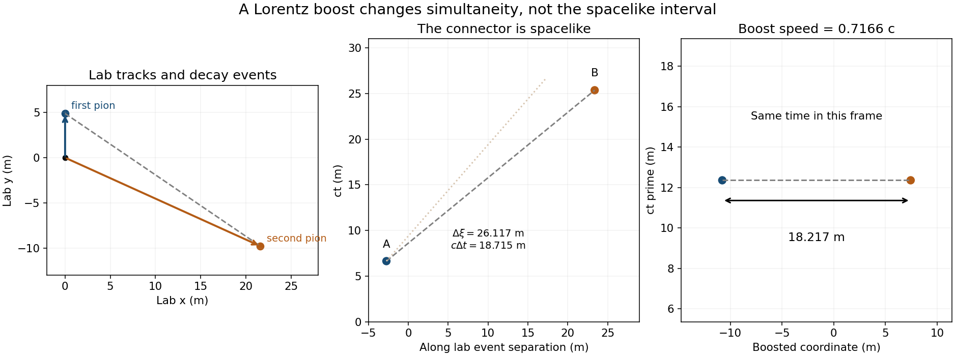
Take the kaon decay as the common origin. A pion traveling freely with constant momentum has lab decay time $t_i=(E_i/m_{\pi }{c}^2){\tau }_i$ and position ${\mathbf{r}}_i=({\mathbf{p}}_i/m_{\pi }){\tau }_i$. The supplied proper survival times therefore giveConsequently the separation from the first decay event to the second isThe requested distance is the separation of the two events, not the sum of the two individual pion path lengths.

Here $|\Delta \mathbf{r}|>c|\Delta t|$, so the separation is a spacelike separation. There is an inertial frame in which the events are simultaneous; in that frame their distance equals the invariant spacelike length:One such frame moves along $\Delta \mathbf{r}$ with $\mathbf{V}=c^2\Delta t\Delta \mathbf{r}/|\Delta \mathbf{r}{|}^2$, of speed $0.71658c$. The simultaneity condition is then $\Delta t^{\prime }={\gamma }_V(\Delta t-\mathbf{V}\cdot \Delta \mathbf{r}/c^2)=0$.

The spacelike distance between daughter decay events provides an independent invariant check: the daughter four-velocity contraction givesIt produces the same distance without using the particular kaon laboratory boost. A simultaneous frame exists only when this expression is positive, as it is for these two survival times.

Maintaining a fixed separation in one inertial laboratory frame is not the same as maintaining a fixed separation measured locally with the accelerating rockets. The attached string is prevented from undergoing the laboratory contraction that an unstrained comoving string would have. It is therefore stretched and develops tensile stress: this is Bell's spaceship paradox, not a failure of Lorentz contraction.

For sufficiently prolonged acceleration and a finite elastic breaking strain, the string breaks. If an acceleration history produces only a small bounded increase in speed, whether it actually breaks depends on its material strength; the kinematic conclusion is stretching, not an unconditional assertion that every arbitrarily weak acceleration must snap every string. Stress also propagates through a real string at a finite speed. The construction enforcing Born rigidity in the following parts is a different set of trajectories chosen to keep the comoving separation fixed.

Let $A=(c{t}_A,f(t_A))$ on the rear rocket and $B=(c{t}_B,h(t_B))$ on the front rocket. The instantaneous inertial rest frame of the rear rocket at $A$ moves at $v=f^{\prime }(t_A)$ relative to S. Transform the time difference of these two events:Setting $\Delta t^{\prime }=0$ givesThe velocity belongs to the rear event $A$. It is not to be evaluated at laboratory time $t_B$, nor does the simultaneity condition mean $t_A=t_B$ in S. At nonzero velocity the front event on the same instantaneous-rest slice is at a different laboratory time.

Use the same event pair already made simultaneous in the rear instantaneous rest frame. Its proper spatial separation is the Minkowski interval length, soThe inequality selects the front rocket rather than the equally long backward extension. Equivalently the Lorentz-transformed spatial difference obeys $\gamma [h(t_B)-f(t_A)-v(t_B-t_A)]=L$. This is not the condition $h(t)-f(t)=L$ at equal laboratory times, which would describe the stretching arrangement in a.

Write $\Delta x=h(t_B)-f(t_A)$. Substituting $\Delta t=v\Delta x/c^2$ into ii gives $L^2=\Delta x^2(1-v^2/c^2)$. The positive-separation branch therefore hasThe Born-rigid front trajectory from a rear worldline follows by setting $t_A=t$:Every $v$ and $\gamma$ in this formula is evaluated at the rear event with laboratory time $t$, not at the shifted argument of $h$.

For completeness, a smooth future-directed front trajectory requires this time mapping to be locally invertible. If the signed laboratory acceleration is $a_S=dv/dt$ and the rear proper acceleration is ${\alpha }_F={\gamma }^3{a}_S$, thenWhen $1+L{\alpha }_F/c^2>0$, their ratio gives $dh/d{t}_B=v$, so the two simultaneous points indeed share their instantaneous velocity. If that factor reaches zero, an acceleration-horizon obstruction appears; an arbitrary rear trajectory cannot be extended to an arbitrary rigid length while retaining both rockets future-directed. The positive-acceleration example below satisfies the condition.

Take $a>0$ as a length. For the rear hyperbola,The implicit front event from iii has $t_B=(1+L/a)t$ and $x_B=(1+L/a)f(t)$. Eliminate the rear time $t$ to obtainThe rear proper acceleration is $c^2/a$, while the front proper acceleration is $c^2/(a+L)$. Thus Born rigidity in the acceleration requires the front rocket to accelerate less strongly. Their constant separation $L$ is measured on the tilted instantaneous-rest slices; their equal-laboratory-time coordinate separation decreases from $L$ rather than staying constant. At $t=0$ both rockets are at rest, at $x=a$ and $x=a+L$.

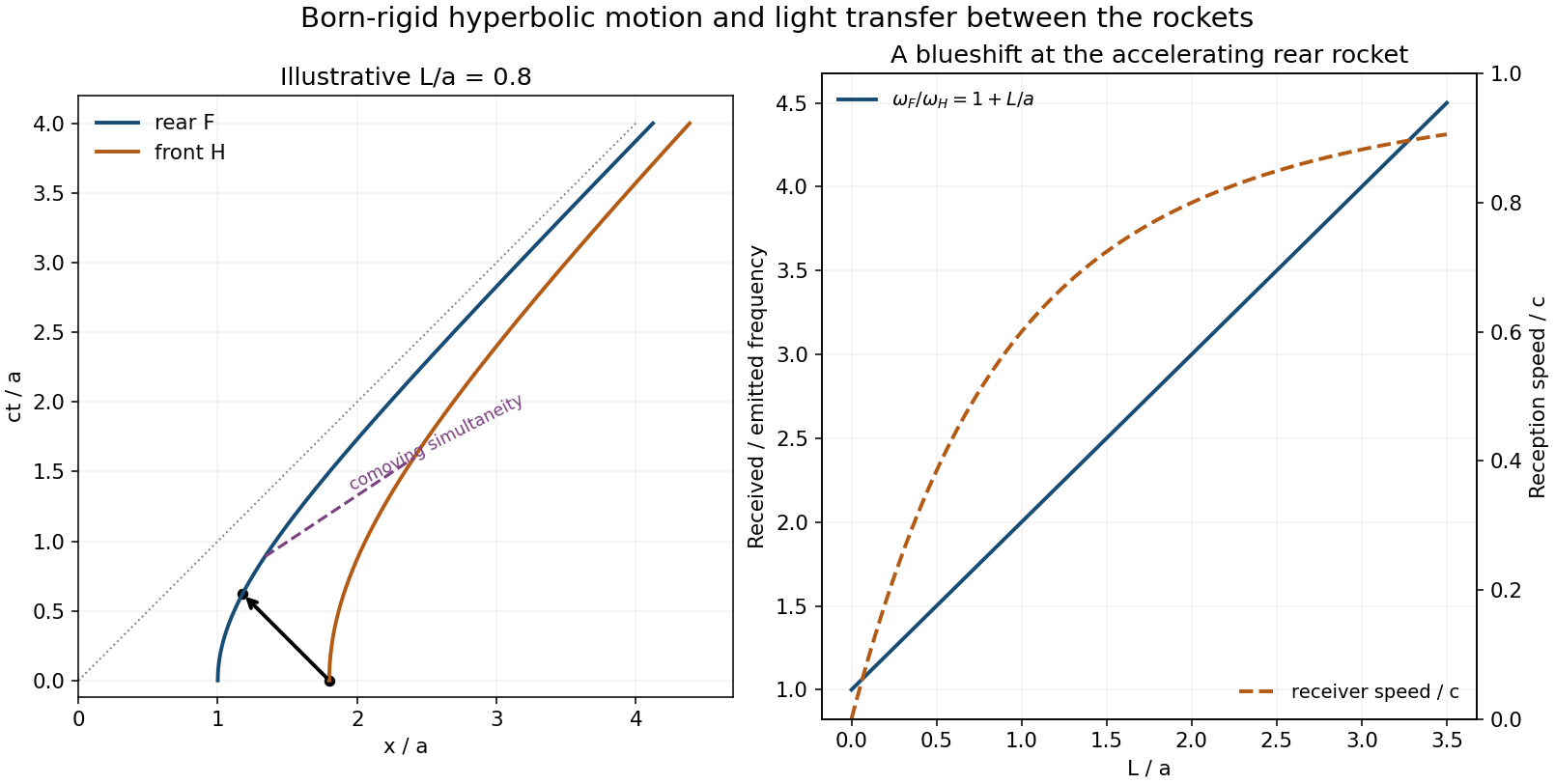
The photon leaves the front rocket at $(t,x)=(0,a+L)$ and moves toward decreasing $x$, so its laboratory path is $x_{\gamma }(t)=a+L-ct$. Intersect it with the rear hyperbola, keeping the future root. Squaring and cancelling $c^2{t}^2$ givesThe rear rocket's speed there isAt emission the front rocket is instantaneously at rest in S, so the photon laboratory frequency is ${\omega }_H$. At reception the rear rocket moves in $+x$ while the photon travels in $-x$. The Doppler factor for this head-on reception isThe receiver sees a blueshift. It is essential to use the front velocity at emission and the rear velocity at reception; comparing the two velocities at one laboratory time would describe the wrong pair of measurements. The result also agrees with the Rindler light-transfer frequency ratio for static accelerated observers at radii $a$ and $a+L$. In the weak-acceleration limit $L/a\ll 1$, the shift is $1+L/a$, and the arrival time approaches $L/c$, providing useful checks.