Source bundle pages 71–75. The cover establishes 2022 despite the attachment filename. Throughout these solutions the metric signature is , as fixed by the source's lowered time coordinate. Question 2 uses . Signs and additional assumptions needed by particular printed conclusions are explained where they arise.
Write the Lorentz transformation as . Acting on a scalar field, the chain rule gives the four-gradientFor the specified Lorentz boost, the inverse is obtained by changing to , soThese are precisely the covector component rules for the lowered coordinates. Raising the index with the Minkowski metric reverses the time component, yieldingIndeed and , the contravariant four-vector rules. Thus the index on a partial derivative with respect to an upper coordinate is lower.
The four-gradient rules from a giveThe Lorentz transformation coefficients are constant, so the partial derivatives do not differentiate them. This proves the Lorentz invariance of the d'Alembert operator:For example, the two longitudinal terms transform as , using and commuting partial derivatives. The transverse terms are unchanged. Applied to a scalar field, therefore gives a Lorentz scalar.
Take the divergence of the Ampère-Maxwell equation and use that the divergence of a curl is zero:The last step uses Gauss's law. Thus the charge continuity equation is exactlyFor a direct justification that this four-current is a four-vector, take one locally comoving population of electric charges, with rest charge density and four-velocity . Invariance of electric charge and length contraction give and , hence . Summing populations preserves the four-vector rule. In particular, and . The Lorentz invariance of its four-divergence then explains why charge conservation holds in every inertial frame. A single zero-divergence condition alone would not determine a field's transformation law; the physical charge density and current density provide the additional content.
The Lorenz gauge condition is . Substitute the electric potential and magnetic vector potential into Gauss's law:Next the Ampère-Maxwell equation, the curl of the curl identity, and the Lorenz gauge condition giveThe gradient terms cancel. Since , the time component obeys , so togetherThe four-potential can be chosen to transform as a four-vector. To make the argument rigorous, choose the retarded potential with no freely added homogeneous solution. If , this choice isThe retarded Green function is a Lorentz scalar under proper orthochronous Lorentz transformations, and is invariant. The four-vector rule for therefore proves . More generally, transform any homogeneous initial data by this same rule. Both the wave equation and the Lorenz gauge condition are then preserved.
Qualification. The wave equation by itself cannot prove the transformation rule for every independently chosen gauge potential: the d'Alembert operator has a nontrivial kernel of a linear map. For a concrete counterexample, zero sources and zero fields admit in one inertial frame and in another. Both satisfy the wave equation and the Lorenz gauge condition, but the latter is not the Lorentz transformation of zero. It is a residual Lorenz gauge symmetry, generated by . Thus the usual assertion is a covariant choice of four-potential, with a consistent gauge transformation and homogeneous data, rather than a uniqueness result from the displayed equation.
Let . The Lorenz gauge condition on the plane electromagnetic wave givesThe vacuum wave equation gives for a nonzero amplitude; equivalently and . Use the gauge transformation withBecause , this is a residual Lorenz gauge symmetry and . For a propagating plane electromagnetic wave, , so take . ThenThe second equality follows from . The electric field and magnetic field are unchanged by this gauge transformation. Thus Lorenz gauge permits a representative in radiation gauge; Lorenz gauge alone does not require the spatial amplitude of every representative to be transverse.
Use and define the total four-momentum . For an inertial frame moving with velocity relative to the laboratory, the Lorentz boost givesChoose parallel to and require zero total three-momentum. ThenThis requires , so that the total four-momentum is timelike. Its invariant mass is , the total relativistic energy in the center-of-momentum frame. If all particles are exactly parallel photons, the total four-momentum is null and no finite-velocity center-of-momentum frame exists.
Sign qualification. The minus sign printed in the source describes the laboratory's velocity in the center-of-momentum frame, or the parameter of an active Lorentz boost with a plus-sign spatial rule. It is not the velocity of the center-of-momentum frame relative to the laboratory under question 1's passive convention. For example, a single particle with has its rest frame moving at . The printed would give , which is not zero. This explicitly resolves the sign rather than assigning a rest frame moving away from the particle.
By four-momentum conservation, . With the Minkowski metric, the neutral pion has , while each photon has and . Taking the Minkowski norm givesThe half-angle identity therefore yieldsThis is a measurement of the diphoton invariant mass using two photon energies and their opening angle, independent of the neutral pion's laboratory velocity.
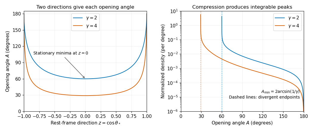
In the center-of-momentum frame, four-momentum conservation gives two opposite photon momenta, each of energy . Let , with the axis along the Lorentz boost from that frame to the laboratory. Reversing the axis specified in the source changes to and has no effect on the following product. The Lorentz transformation of four-momentum givesWriting , b now impliesThe isotropy assumption is on . Each interior opening angle has two inverse branches, and , both of which must enter the change of variables for probability densities. The positive branch has derivativeConsequently the diphoton opening-angle distribution isIts support is for , and its integral is , the integral of the original angular probability density before normalization. Thus the normalized probability density is . Omitting one inverse branch would incorrectly halve the total count.
From c, , with equality when : the photons are emitted perpendicular to the Lorentz boost axis in the center-of-momentum frame. ThereforeAt the minimum, the map is stationary: writing , its leading behavior is . A nonzero interval of uniformly distributed is therefore compressed near , producing an integrable inverse-square-root singularity in the opening-angle probability density. No differentiation of that probability density is needed. For finite , the probability density vanishes at . For the center-of-momentum frame is the laboratory and every event has : the probability distribution becomes a Dirac delta distribution, rather than the singular substitution in c. At large , in radians.

For a massive particle, the proper time is determined by the Minkowski interval along its worldline:Choose future-directed time increments. With the Lorentz factor ,We use for the source's to distinguish four-velocity from velocity . Since proper time is invariant and is a four-vector, is a four-vector, with . The rest-frame result follows immediately.
The Lorentz boost from A to B givesDivide each spatial displacement by . The velocity-addition formula isThe same result follows by transforming the four-velocity and using . The transverse velocities change because the transformed time increment depends on , even though the transverse spatial coordinates are unchanged.
For , decompose the velocity as , parallel and perpendicular to . A rotation-free Lorentz boost gives the velocity-addition formulaThese two components are orthogonal, soThe last equality is Lagrange's identity for the cross product. For physical subluminal speeds, , givingThe case follows directly or by continuity. An independent form useful for checks is , obtained from the transformed four-velocity normalization.
Let and in A. Each has Lorentz factor . The relative Lorentz factor of in the rest frame of follows from their four-velocity tensor contraction:Let be the relative speed divided by . In the rest frame of , take between the photon's propagation direction and 's velocity. The observed angular frequency is the invariant . Applying it to the emitter, whose rest angular frequency is , gives . Since ,This is a relativistic Doppler effect calculation using both emitters' and receivers' rest clocks; the time delay of reception introduces no extra factor for constant velocities.
For the direction in A, write the wave four-vector as , where is a unit vector. Equality of the emitted and received angular frequencies gives . Since the two laboratory Lorentz factors are equal, their time components cancel:Thus the complete answer in three spatial dimensions isIf propagation is additionally assumed to lie in the stars' motion plane, this reduces to either direction along the internal angle bisector, or from . Reflection exchanging the stars' laboratory velocities explains the angle bisector by symmetry. The source does not specify coplanar propagation or the stars' positions, so it does not fix the sign or exclude an out-of-plane ray. For example gives and satisfies the same no-shift condition. Initial positions can be chosen to make such a ray connect emission and reception. All these possibilities give the same rest-frame above.
For constant laboratory force and initial rest, integration gives three-momentum . The energy–momentum relation gives , and , soFor and , its speed increases monotonically, is strictly below the speed of light at every finite time, and obeys . Thus is the limiting supremum, rather than a speed attained at a finite time. The degenerate case leaves the particle at rest and does not have this limit.
With constant rest mass, and the chain rule gives . Hence the laboratory relativistic force isUse the vector triple product identity , and , to obtainThe relativistic energy is , whose time derivative is . Taking the dot product of the first expression for with gives the same quantity, because . Thus . Since , the four-force isIts tensor contraction with the four-velocity vanishes: . This orthogonality also follows by differentiating . Resolving the laboratory acceleration relative to gives and .
Metric-sign qualification. With this paper's metric signature, b givesThe minus sign in the printed Larmor formula would therefore make a positive radiative loss negative. A concrete counterexample is an instant of rest with nonzero acceleration: , so the printed expression is . That sign is appropriate for the opposite metric signature. With the convention already fixed in question 1, positive emitted power instead isAlternatively the printed negative quantity can be interpreted as the particle's signed radiative energy change, rather than the positive loss magnitude.
For fixed rest mass, resolve the acceleration parallel and perpendicular to the velocity, as in b. This givesWriting , the Liénard radiated-power formula becomes . For uniform circular motion, the acceleration is perpendicular to the velocity; for straight-line motion it is parallel. Comparing the same particle at equal relativistic energy and equal laboratory acceleration magnitude therefore givesThis particular comparison makes the linear loss larger. The familiar larger loss from bending applies to a different comparison: at equal applied laboratory force magnitude , and , giving and . Stating which quantity is held fixed is essential.
Both the muon and electron have the same electric charge magnitude. At equal kinetic energy per particle, their Lorentz factors are , so the heavier muon has the smaller Lorentz factor. At equal total relativistic energy the same ordering follows from , provided that energy is large enough to create either particle.
If the equal-acceleration comparison of c is retained, . Thus the four-way instantaneous comparison selectsFor positive , its smaller Lorentz factor reduces the power relative to an electron, and transverse acceleration reduces the power relative to longitudinal acceleration of the same magnitude. This conclusion follows from the constraint actually stated in c.
For the customary engineering comparison at equal applied force, the result changes. From c,Under that comparison the choice isIts longitudinal radiative power is smaller than an electron's by , while avoiding bending removes the extra factor. At a fixed bend radius , the circular loss is , giving the familiar suppression at fixed ultrarelativistic energy and .
An energy budget alone does not specify a unique optimization. The force, acceleration, bend radius, acceleration time, and length are otherwise unrestricted. For example, in a linear accelerator a constant small force gives radiative power proportional to , and reaching a specified final three-momentum takes time proportional to ; the total radiated energy therefore tends to zero as . One cannot infer a unique accelerator choice without an additional constraint. The standard practical preference is the second boxed answer, with its stated comparison. Muon decay introduces a separate lifetime constraint if slow acceleration is contemplated, but it was not part of the specified radiative-loss calculation.
Source bundle pages 70–73; the cover identifies Trinity Term 2021 despite the attachment filename. Use coordinates , metric signature , and . For the electromagnetic field tensor use and . Prescribed external fields are treated classically, neglecting radiation reaction in the trajectories; radiation losses are computed separately where requested.
Let be the magnitude of the electron's electric charge, , , and . The Lorentz force is , so the electron and Positron acquire opposite momenta:Using the relativistic energy-momentum relation, , and integrating from rest gives the world linesFor , the world lines are vertical at on a spacetime diagram. They join smoothly to the accelerated branches with zero initial velocity. At small , and ; at large , their velocities approach , respectively. Each accelerated world line is a branch of a hyperbola, since and . The electric field separates the opposite electric charges in this orientation. The asymptotes are lightlike, while every finite-time tangent is timelike.
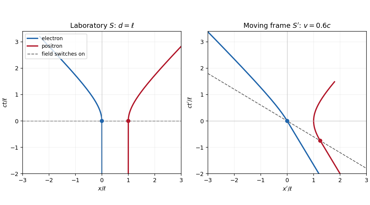

Write for the Lorentz factor of the inertial frame , distinguishing it from the particles' changing Lorentz factors. Apply the Lorentz transformationto each world line in a. Both particles initially have velocity in . The switching events have coordinatesThus the Positron starts accelerating earlier in . Its velocity first becomes less negative, vanishes when its laboratory velocity reaches , and then becomes positive. The electron continues at until , then accelerates toward . The relativistic velocity-addition formula makes this precise:The electric field parallel to the Lorentz boost has unchanged magnitude, but its switching surface is , rather than everywhere.
In the laboratory, the total three-momentum is zero for all : the two Lorentz forces cancel at equal laboratory times. In , each active force is still , since this is one-dimensional motion with a parallel electric field. Define . For the total three-momentum, evaluated at equal , isThis follows by integrating from its switching event and from its later switching event. During the interval between them only the Positron feels the prescribed electric field, so momentum conservation for the particle pair fails. Once both forces act, the total three-momentum is constant again.
The equal-time momentum of an externally driven particle pair illustrates a distinction. The sum of particle four-momenta at a fixed pair of events is always a four-vector. However, a fresh sum at equal time in each inertial frame generally uses different events. Here transforming an equal- laboratory sum would give , which varies with ; this differs from the equal- answer above. For example, with and , the late-time equal- sum is , whereas transforming the equal- sum gives . This is a concrete failure of treating the pair's equal-time sums as components of a single frame-independent four-vector.
A closed system's total four-momentum, including the electromagnetic field and the apparatus supplying it, is conserved and independent of the choice of spacelike integration surface under the usual isolated-system boundary conditions. The particles alone exchange energy and momentum with an external system, so neither that independence nor universal particle-only momentum conservation is guaranteed.
With the reversed electric field, reflection about exchanges the electron and Positron. They therefore meet there with equal and opposite momenta. Each travels , and the work-energy theorem gives its kinetic energy:Their combined kinetic energy is , while each total relativistic energy is . The laboratory is the center-of-momentum frame of the colliding pair.
Local four-momentum conservation in the electron-positron annihilation excludes one real photon: the incoming total four-momentum is timelike, with zero spatial component and positive energy, while a single photon's four-momentum is null and has . Two photons can balance their momenta by travelling in opposite directions, soThe equal photon energies follow from opposite equal momenta, not merely from sharing the incoming energy arbitrarily. Here . This is the free local annihilation idealization implicit in the question; significant momentum transfer to the external apparatus would change the kinematic system being considered.
The laboratory remains the center-of-momentum frame. At the relativistic collision mass threshold, the two final W bosons can have arbitrarily small opposite momenta. The available relativistic energy is , soEach incoming particle must acquire about of kinetic energy, travelling about . Equality is the ideal kinematic threshold; a nonzero production rate needs energy above it. This estimate neglects acceleration losses and treats the W bosons with the supplied nominal rest mass.
A linear particle accelerator avoids repeatedly bending high-energy electrons and Positrons. This greatly reduces the bending synchrotron radiation loss, which at fixed bending radius grows approximately as the fourth power of the relativistic energy for a given particle species. Its useful collision energy can therefore be increased without the severe circular electron collider radiation penalty. The price is long structures or high accelerating gradients: each bunch normally passes once, requiring substantial beam power, fresh bunches, and very tight focusing for high luminosity. A circular particle accelerator reuses its accelerating structures and circulates bunches through many collisions, but needs a large ring and substantial radiofrequency power to replace synchrotron radiation losses. Heavier particles such as protons radiate far less at a given energy and radius, although a proton's constituent structure makes the hard-collision energy less sharply specified than in an electron-positron annihilation experiment.
Let be the point electric charge's world line, with proper time and four-velocity . For the field event , choose the retarded source event: is future-directed and null. Write , where . In the instantaneous rest inertial frame of that source event,Consequently the covariant expression matching this Coulomb potential isThe denominator is a Lorentz scalar, so the right-hand side is a four-vector with the required instantaneous-rest components. This describes the retarded potential in Lorenz gauge, with no added free electromagnetic wave. Lorentz covariance alone does not establish the boundary conditions or exclude additional terms depending on four-acceleration. The physical input is the retarded point-source solution of Maxwell equations: the potential at the retarded event depends on the instantaneous four-current, while its derivatives generate the acceleration field. Equivalently, evaluating the retarded source integral gives a Jacobian from the light-cone constraint; this fixes that input for arbitrary smooth subluminal motion.[ref]
Retarded Potentials by Richard Fitzpatrick. §1.7, equations (71)–(76): causal source integrals, with source quantities evaluated at retarded time
In any inertial frame, put and . Then , and the Liénard–Wiechert potential isDifferentiate using and , including the position and time dependence of the retarded time. For example, and . The resulting Liénard-Wiechert field isHere the dot denotes a derivative with respect to source coordinate time. The first term is the velocity or non-radiative field: it falls as and exists even without acceleration. The second is the acceleration or radiation field, falling as and transverse to . Its Poynting flux falls as , so its outward power integrated over a large sphere stays finite as its radius tends to infinity. The first term's squared-field flux instead vanishes in that limit. This large-distance distinction defines radiation; a moving near field can carry local energy without constituting radiation escaping to infinity.
For uniform circular motion, the transverse Lorentz force supplies the change in direction of three-momentum:The magnetic rigidity relation gives . Using ,The coordinate centripetal acceleration is . For transverse acceleration, the magnitude of the four-acceleration, or proper acceleration, is . The supplied Larmor formula, in its proper acceleration form, therefore givesThe emitted power here is also the laboratory total emitted power: in the instantaneous rest inertial frame the dipole radiation pattern has zero net radiated three-momentum, so both emitted energy and elapsed coordinate time gain the same Lorentz factor on transformation. This does not assert that a directional detector flux is invariant.
Numerically , per electron, andThe synchrotron's radiofrequency accelerating system must replace this lost energy to keep and magnetic rigidity fixed over many revolutions. The fraction lost per turn is about , so a fixed-orbit calculation over one turn is self-consistent.[ref]
Synchrotron Radiation by Richard Fitzpatrick. §12.22, equations (1975)–(1978): transverse radiated power and energy per revolution
For an ultrarelativistic particle, relativistic beaming concentrates the synchrotron radiation within an angle of order around its instantaneous velocity. A fixed viewing direction in the orbital plane receives an intense signal only when the tangent sweeps through that direction. One electron, or one sufficiently short bunch, therefore produces one pulse per revolution, separated by . Several bunches produce the corresponding additional pulses per revolution.
The time during which the velocity points within that cone is of order , but this is the emission interval. If is the arrival time at a distant detector,Near alignment, . Thus synchrotron pulse compression reduces the observed duration by a further factor of order :A more explicit geometric estimate chooses the cone edges . With , along the line of sight, the difference in arrival-time compression for a moving source isThe order-one coefficient depends on how pulse width is defined; the robust scale is . The usual central-cone estimate gives . These estimates agree on the attosecond scale and must not be confused with .[ref]
Synchrotron Radiation by Richard Fitzpatrick. §12.22, equations (1979)–(1981): distinction between emission interval and detector arrival interval
Bunch qualification. The source says only that the bunches are short, without their longitudinal length . Different electrons pass the same emitting tangent at times separated by up to about , with essentially the same path length from that tangent to the detector. The bunch-length broadening of synchrotron radiation means that the measured bunch envelope is the single-electron pulse convolved with the bunch's passage-time profile; its scale is generally at least of order , with additional detector bandwidth effects. For example, a bunch, very short compared with this ring, gives an approximately envelope, much longer than the single-electron duration. No unique numerical bunch-envelope width follows from the supplied data. The pulse argument also presumes that the accepted direction is tangent to the orbit; a direction far outside the orbital plane receives no comparable intense forward pulse.
Assume for the directions and parametrizations; the boost formulas retain their signed meaning for reversed fields. A Lorentz boost with velocity along transforms the transverse electric field and magnetic field asIn the electric-dominated case chooseThe inequality ensures , so this is an inertial frame. The field-removing boosts for perpendicular electric and magnetic fields are governed by the electromagnetic field invariants and explain why a purely electric inertial frame exists and a purely magnetic one does not.
The electron is not initially at rest in this convenient inertial frame: its initial velocity is and its initial three-momentum is . Thereafter , while stays constant. The electric field accelerates it toward ; as its relativistic energy increases, its negative transverse velocity decreases in magnitude. Defining and gives a useful parametric world line:Here is the proper time. These formulas follow by integrating , , and constant . Its projection onto the plane is a hyperbola, but the spatial trajectory includes the initial transverse motion and is not a straight line.
Transforming back with , givesThe laboratory trajectory starts from rest toward , then bends toward . It is unbounded in and ultimately has and . Thus the late velocity has magnitude as a limit, consistent with the relativistic energy-momentum relation, rather than undergoing a closed cyclotron orbit.
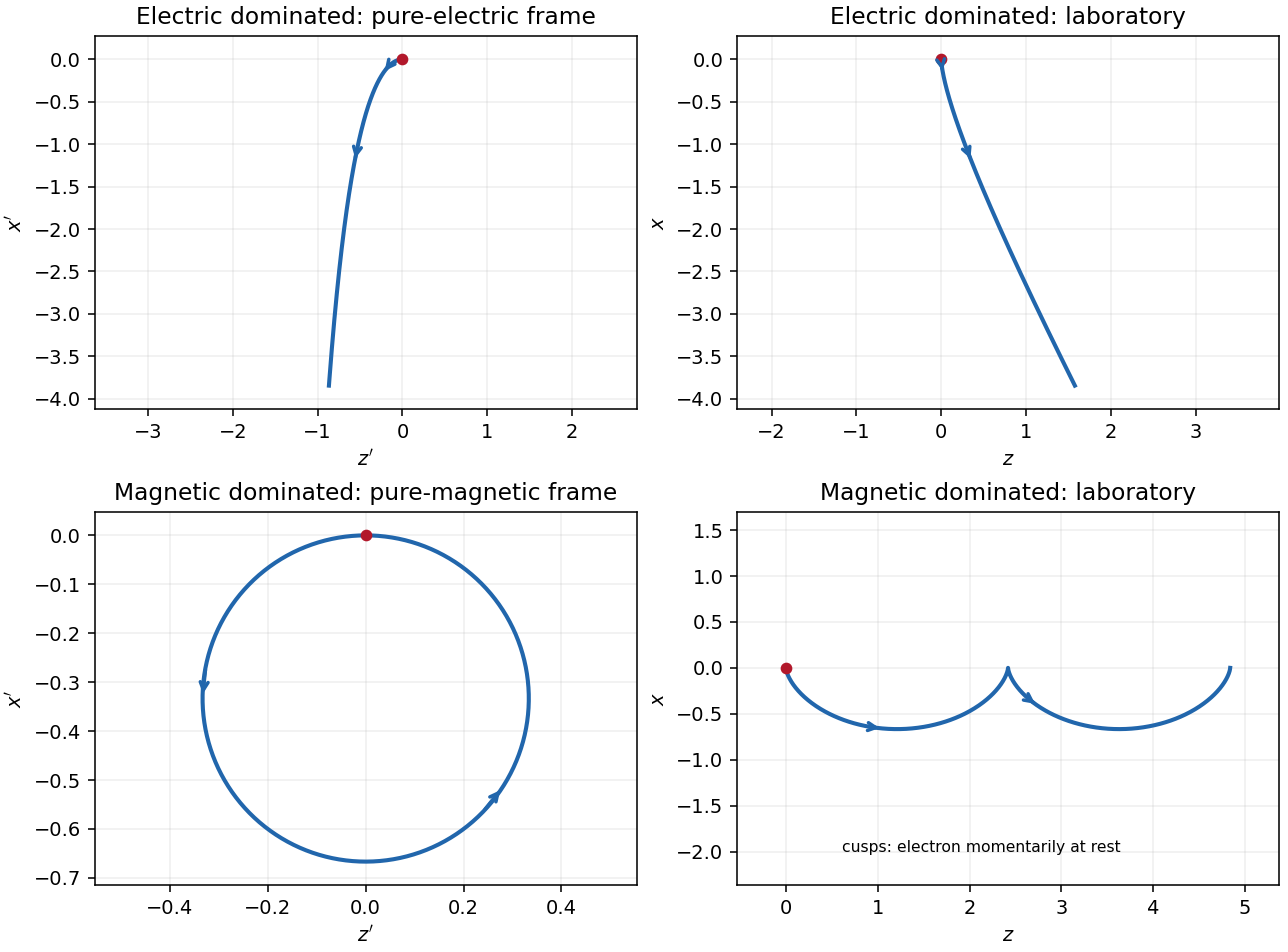

In the magnetic-dominated case the suitable Lorentz boost instead hasThe hypothesis gives . The electromagnetic field invariants now have , allowing a purely magnetic inertial frame. The initial velocity is again , perpendicular to . Since a magnetic field does no work, the electron's relativistic energy and speed in this inertial frame remain constant. Its trajectory is a circle in the plane with Lorentz factor and cyclotron frequency .
For , set and . A parametrization with the correct initial velocity and Lorentz force isTransforming the world line back to the laboratory givesThe laboratory trajectory is a stretched cycloid, with cusps at where the electron is momentarily at rest. It first accelerates toward , then curves toward , returning to its original coordinate each cycle while advancing in . Its mean drift is , the E-cross-B drift. Its laboratory kinetic energy oscillates as the electric field does positive and then negative work; it does not grow indefinitely. The strict inequalities in the two branches exclude the null case , where neither field can be removed by a finite Lorentz boost.
Use the electromagnetic field tensor convention stated above, and lower indices with the Minkowski metric . Lowering a single time index changes its sign. Summing both orders of each antisymmetric index pair gives the Lorentz scalarFor , and . Direct substitution in the printed electromagnetic stress-energy tensor yieldsFor a spatial index , and . HenceThus the full top row isHere is the electromagnetic energy density and the Poynting vector, using . By the symmetry , these components describe both energy flux divided by and times the electromagnetic momentum density . Keeping the factor is essential because the time coordinate is .
Let starred quantities denote the capacitor's rest inertial frame, , , and . Work in the uniform interplate region of an ideal parallel-plate capacitor, neglecting its fringing field of a capacitor. To transform from that rest inertial frame to a laboratory in which the capacitor moves along , use the positive-sign Lorentz transformationFor a purely electric field, the spatial block of the electromagnetic stress-energy tensor isThis is the negative of the Maxwell stress tensor: it has along the electric field and perpendicular to it. The stress contribution to energy transport in a moving capacitor is essential to the Lorentz transformation of the energy density and flux.
Plates parallel to . Choose and . The electromagnetic field tensor and electromagnetic stress-energy tensor areThe transformed nonzero independent electromagnetic field tensor components are and . Thus and , consistent with . Transforming the electromagnetic stress-energy tensor givesIn particular, the laboratory Poynting vector is , and the electromagnetic energy density is . The ratio is subluminal for , but differs from the capacitor's velocity. The difference from a simple convective flux isThe extra term is , the rest-frame stress multiplied by the velocity. This shows why treating stored field energy as an unstressed parcel moving rigidly with the plates misses part of the energy transport.
Plates parallel to . Now . The rest tensors areThe electric field is parallel to the Lorentz boost, so remains unchanged and . The cancellation between and givesThere is no Poynting flux in the ideal interior in this orientation, although the region containing the electric field moves. The longitudinal negative stress contribution cancels the convective term: . Field energy is removed at the receding boundary and supplied at the advancing boundary by work on the charged plates; it need not flow through the interior to accompany the moving region. At edges, omitted fringing fields provide additional local structure.
For a finite idealized interplate rest volume , length contraction gives . The field-only integrated laboratory energies would consequently be and , with . Their different transformation laws are not paradoxical: the field alone is not a closed system. Include the plates and the supports holding them apart, whose mechanical stresses balance the Maxwell stress tensor. The total closed-system four-momentum then has the ordinary Lorentz transformation law. This is the same distinction between a subsystem and a conserved whole that appears in b.
A symmetry is a transformation of a physical system that preserves its laws: it maps admissible solutions and consistently transformed data to admissible solutions. The central symmetry of special relativity is Lorentz invariance, expressing equivalence of inertial frames and preservation of the Minkowski interval and the universal speed of light. With spacetime translations included, the spacetime symmetry group is the Poincaré group.
A practical sufficient check is to express an equation as an equality between Lorentz tensors of the same type, with every repeated upper/lower pair correctly contracted and the same free indices on both sides. Every ingredient, including sources and background fields, must have its stated Lorentz transformation rule. For example, is a Lorentz scalar equality, and equates four-vectors. Such manifest Lorentz covariance makes the form of the equation the same in every inertial frame.
This is a sufficient test when the transformation rules are genuine physical ones, not a guarantee from writing index symbols. A fixed preferred four-vector could make an equation formally covariant if it too were transformed, while its chosen physical background breaks Lorentz invariance. Conversely, an equation written in three-dimensional components can be fully consistent with special relativity, as the Lorentz force is, even when the covariance is not manifest.
For an active clockwise rotation of column vectors in the usual oriented plane, takeDirect matrix multiplication givesThus the rotation matrix is an orthogonal matrix, preserving the Euclidean inner product, with determinant .
For a passive one-dimensional Lorentz boost, use rapidity , :This is not unless . Hence a nontrivial Lorentz boost is not an orthogonal matrix for the Euclidean inner product. Instead it preserves the Minkowski metric:by . Thus it is pseudo-orthogonal. The zero-rapidity identity is the explicit exception to the assertion that a Lorentz boost is not orthogonal.
The supplied matrix obeysSeparate the even and odd powers in the matrix exponential to obtainIt fixes the component and is a counterclockwise active rotation viewed from . This sign differs from the clockwise convention in b, because the source fixes the sign of both and the exponential. Replacing by yields the clockwise rotation.
With , the generators of rotations obeyThe commutator measures the leading difference between performing two infinitesimal rotations in opposite orders. For example, with and ,The failure to commute is itself an infinitesimal rotation about the perpendicular axis; the Lie algebra closes on the same three generators of rotations.
To pass from this local statement to the full group property, put . These are real antisymmetric matrices, with . The Baker--Campbell--Hausdorff formula shows locally that the logarithm of a product of their exponentials remains a linear combination of the , because all nested commutators do. Globally, each exponential has and . If have these properties, thenEvery real three-dimensional orthogonal matrix of determinant has an eigenvector with eigenvalue : its nonreal eigenvalues come in conjugate pairs, and the product of all three is . On the perpendicular plane it acts as a two-dimensional rotation. It therefore has axis-angle form and can be written . Thus the product is again a rotation. The identity is , the inverse reverses , and associativity comes from matrix multiplication. This proves that all these rotations form the special orthogonal group . The commutator supplies local closure, while the orthogonality and axis-angle argument supplies the necessary global step.
Let generate Lorentz boosts with the same exponential convention as the rotation generators of rotations . The Lie algebra of the Lorentz group isConsequently non-collinear Lorentz boosts do not close among themselves: the product contains a rotation, the Wigner rotation. For an explicit counterexample, in coordinates write , and similarly for . ThenA pure rotationless Lorentz boost has a symmetric matrix, whereas this product has spatial entries and for . It is therefore a concrete product of two pure Lorentz boosts that is not a pure Lorentz boost. Collinear Lorentz boosts are the special case that do form a one-parameter group, with additive rapidities.
Allowing all spatial directions and closure generates both the and, through their commutators, all . The smallest connected group containing all these Lorentz boosts is the proper orthochronous Lorentz groupIt contains arbitrary compositions of spatial rotations and Lorentz boosts continuously connected to the identity. It has six continuous parameters. Here “smallest” refers to the subgroup generated by all continuous pure Lorentz boosts, not to an arbitrary collection already including discrete reversals.
The full Lorentz group has four connected components, distinguished by the sign of the determinant and the direction of time. Representatives are the identity, parity , time reversal , and . ThusMultiplication by these discrete transformations relates the components algebraically; no continuous path within the Lorentz group joins different components. Translations are not required for closure here; adding them gives the larger Poincaré group.
Use coordinates and the mostly-plus Minkowski metric . Along a future-directed timelike world line, proper time satisfiesThe four-velocity and four-acceleration areThe Minkowski norm is fixed: . Differentiating with respect to proper time, using the constant Minkowski metric, givesIn the instantaneous rest reference frame, , so the orthogonality says there. This construction uses a timelike world line; a massless particle has no rest-frame proper time parameter.
Let denote the constant rest mass, set , and put . The relativistic three-force is , soIt follows thatIntegrating the velocity with the initial position fixed givesThese formulas allow either sign of ; their limit is rest at the origin. For , the trajectory obeysThis is hyperbolic motion. Its coordinate acceleration decreases while its proper acceleration has constant magnitude . In particular, a constant three-force does not give constant coordinate acceleration at relativistic speed.
The upper-left panel shows the three causal structure regions, with null boundaries included in the appropriate causal future and causal past. For the charged trajectory, use part b with , choosing the direction so that . The electric field gives the constant three-force and hence the shifted hyperbolaIt starts with a vertical tangent at the origin, stays strictly inside the future light cone, and asymptotes to . The other panels implement the coordinate and topology changes used below; they are original spacetime diagrams, not copies of source artwork.
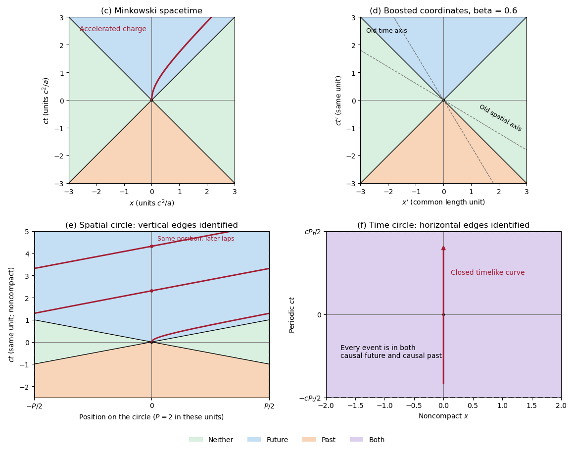
Causal regions in Minkowski spacetime and in spatially or temporally periodic flat spacetimes
. Blue denotes the causal future, orange the causal past, green events in neither, and purple membership in both. The top panels use ordinary and boosted inertial coordinates. The spatial quotient identifies vertical edges and shows the accelerated worldline wrapping across them. The temporal quotient identifies horizontal edges; every event belongs to both causal sets. Details.
A future-directed causal curve from the origin has . Integrating this inequality gives the causal futureThe straight timelike or null segment proves sufficiency. This is the blue region above the two null rays in the upper-left spacetime diagram of part c.
Reverse the endpoints of the future-directed causal curve. The origin can be reached precisely from its causal past,This is the orange region below the two null rays in part c. The origin itself belongs to both the causal future and causal past by the usual zero-length-curve convention.
Outside both light cones, the separation from the origin is spacelike. Thus the events in neither the causal past nor the causal future areNo causal curve can connect either endpoint to the other. These are the two green side regions in part c; the strict inequality excludes the causally reachable null boundaries.
For the standard passive Lorentz boost, write andA proper orthochronous Lorentz transformation preserves the sign of the time component of a nonzero future causal vector and preserves its Minkowski norm. ThereforeThe upper-right panel of part c uses horizontally and vertically. Its null rays still have slopes . The grey dashed old axes satisfy for the old time axis and for the old spatial axis; changing the coordinate grid has not changed which events are reachable.
The same Lorentz transformation maps the past light cone to itself. In the primed axes the causal past isthe orange region in the upper-right spacetime diagram of part c. Future and past are not interchanged by the standard boost.
The invariant spacelike condition is . Hence the primed-coordinate events in neither the causal future nor the causal past obeyThe green regions in part c retain their shape in primed coordinates. A particular spacelike event's coordinate time may change sign, but it never enters either light cone.
For causal reachability on a spatial circle, put and use a representative of the spatial circle. The lower-left panel of part c is a fundamental strip with its vertical edges identified. On the covering space the charged world line is still the solution of part b; on the quotient it isA jump between opposite strip edges is a coordinate seam, not a discontinuity of the physical world line. At its th complete lap, , soFor , the speed increases on each return while remaining below . Its kinetic energy increases byThere is no single-valued electrostatic potential energy on a circle: the nonzero electromotive force is . A globally defined magnetic vector potential one-form instead makes the driving explicit. In an embedded circuit, Faraday's law realizes this electromotive force through changing magnetic flux. More generally an external apparatus maintaining the field supplies the increasing particle energy. In an isolated dynamical field-plus-particle system, backreaction would change the field. Thus this is not a cyclic machine extracting work from a conservative potential, and it does not violate conservation of energy.
A causal curve can wind around the spatial circle. Lift its endpoint to on the covering space. A lift is reachable from the origin if for at least one integer . With shortest circular distancethe causal future isIn the centred fundamental strip, . For , every spatial point is in the causal future. This produces the fully blue upper part of the lower-left panel in part c.
Articles were limited to the first 100 out of 306 total.
Articles by others on the same topic
There are currently no matching articles.