Choose a coarse-grained magnetization as the order parameter: it vanishes in the paramagnetism phase and develops a spontaneous nonzero value in the ferromagnetism phase. In zero applied magnetic field, spin reversal sends , so the local Landau free energy contains only even powers. A minimal spatially inhomogeneous free-energy functional isThe positive gradient coefficient penalizes rapid spatial variations. Near an ordinary transition take , , and positive ; retain the sextic term when can approach or cross zero. The source is conjugate to the magnetization and explicitly breaks spin reversal.
Determine equilibrium by minimizing this free-energy functional, imposing the appropriate boundary conditions. Its Euler-Lagrange equation isFor a uniform system at , compare the values of all stable stationary solutions, rather than accepting every solution of this equation. The selected global minimum gives the equilibrium magnetization; derivatives of its free energy give entropy, heat capacity and magnetic susceptibility. At an ordinary transition the two ordered minima emerge continuously from zero. Spatial dependence also permits domain walls and an estimate of the correlation length.
This is a mean-field approximation: it selects a minimizing profile and neglects statistical fluctuations around it. The symmetry constrains the expansion, but its numerical coefficients are phenomenological. Close enough to a transition, thermal fluctuations near a critical point can invalidate the resulting mean-field critical exponents.[ref]
Statistical Field Theory by David Tong. Chapter 1, the Landau-Ginzburg free-energy functional, spatial gradients and mean-field phase transitions
For the sextic polynomial to be bounded below at large while allowing either sign of , its leading coefficient must obeyIf , the free energy tends to as , so it cannot define an equilibrium within this truncation. The exceptional case is stable for and gives the ordinary quartic Landau theory; it cannot stabilize the negative- region required for the full sextic phase diagram. Higher positive powers could stabilize a negative , but they are absent from this model.
Fix . Stationary points satisfy . With , the nonzero candidates areKeep only real positive roots. At such a point,so gives local minima and gives local maxima when both exist. The solution is a local minimum for . To choose the phase, compare free energies: using the stationary point relation givesFor , this expression is negative whenever a nonzero stationary minimum exists. The paramagnetism phase is stable for , and the ferromagnetism phase with is stable for . The phase transition at , , is continuous and second order.
For , equality with requires . Substitution into the stationary equation gives the first-order coexistence curveThe disordered phase is the global minimum above this curve, and the ordered phase is the global minimum below it. At coexistence the factorizationexhibits three equally low minima, and , proving the discontinuous jump.
The ordered spinodal is , , where its local minimum meets the intervening local maximum. The disordered spinodal is , . Thus the ordered phase is metastable for ; the disordered phase is metastable for . These spinodals are limits of metastability, not equilibrium transition curves.
The first-order curve meets the continuous transition line at the tricritical point . On the specially tuned path , the equilibrium ordered solution is for and tends continuously to zero at the origin.
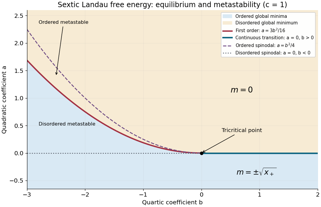
Phase diagram of the sextic Landau free energy, including coexistence, spinodals and the tricritical point
. Details. 
Write , , at fixed , and define the critical exponent by on the ordered side. For fixed and small negative , the stationary equation gives . ConsequentlyAt the tricritical point approached along the tuned path , the stationary equation instead gives , soFor fixed , the transition occurs before reaches zero and the magnetization jumps; it is not a second-order transition and has no vanishing-order-parameter exponent of this form. A path that does not keep the quartic coefficient tuned to zero generally crosses over to the ordinary result.
Take and hold fixed. The heat capacity comes from the minimized free energy, , with any smooth background added separately. For and ,Above , and the polynomial contributes zero. There is a finite jump, rather than a divergence: the conventional ordinary mean-field critical exponents areThe upper branch has zero order-parameter contribution; a finite regular heat capacity has exponent zero.
Along the tuned tricritical path , the ordered minimum givesUpper-side qualification: the vanishing disordered-side heat-capacity amplitude in Landau theory matters here: for and , the minimizing solution is still exactly , so this saddle-point polynomial gives and . A zero function cannot determine a nonzero-amplitude power-law exponent. For example, adding the allowed smooth background , with , leaves the entire phase diagram unchanged but makes the upper-side heat capacity exactly , not a divergence.
One convention assigns the tricritical scaling exponent to both sides, writing with at this mean-field approximation saddle. If the source's literal is meant to have a nonzero leading coefficient, the given polynomial establishes no upper-side tricritical singular exponent; with a nonzero smooth background its leading upper-side exponent is zero. A nonzero upper-side singularity requires fluctuation information beyond this minimization. This distinction prevents claiming an upper-side divergence that the displayed Landau free energy does not produce.
Articles by others on the same topic
There are currently no matching articles.