Source paper: www.whatdotheyknow.com/request/oxford_physics_past_papers_2/response/2340696/attach/6/Physics%20Papers%202017.pdf?cookie_passthrough=1. The cover identifies Trinity Term 2018; the annual bundle's 2017 filename does not determine the examination year. We use natural units for the classical field theory and quantum field theory in four spacetime dimensions and Minkowski metric .
The Euler-Lagrange equation for the real scalar field givesThus the conjugate momentum and Hamiltonian density areThe spatial Fourier transform reduces the Klein-Gordon equation to , with positive frequency . Hence a general real solution is the mode expansion of a free fieldThe two coefficients are complex conjugates because the field is real. Each pair of initial data fixes these coefficients. The normalization anticipates canonical quantization and the relativistic normalization of one-particle states.
Promote the mode expansion of a free field coefficients to annihilation operators and creation operators, replacing by . The canonical commutation relations areTogether with the normalization in part a, they give and vanishing equal-time commutators between two fields or two conjugate momenta.
Insert the mode expansion of a free field in the Hamiltonian. The spatial integral produces . The and coefficients cancel because . The remaining terms giveThis is a continuum of quantum harmonic oscillators. In a finite periodic volume , . The Fock vacuum satisfies , so its vacuum energy density isNormal ordering would subtract this constant; here it must be retained because it is the quantity being calculated.[ref]
Quantum Field Theory by David Tong. Section 2, canonical quantization of the real scalar field and its zero-point Hamiltonian
A spherical three-momentum ultraviolet cutoff givesFor and , the asymptotic expansion isIn particular, the leading ultraviolet divergence is quartic. For , exactly.
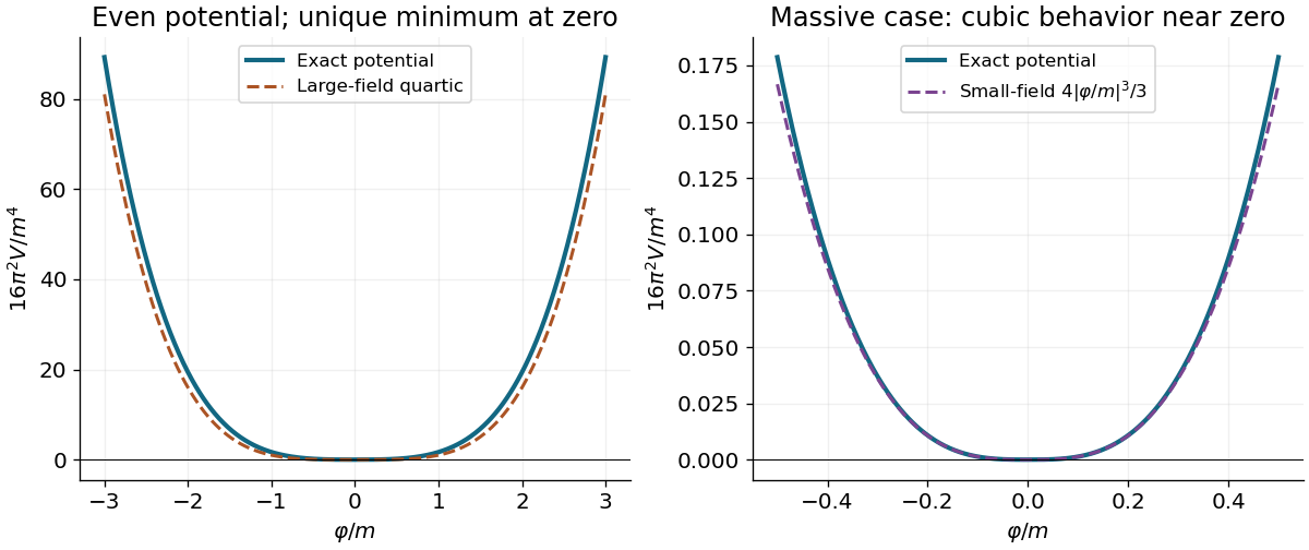
Write . Under the proposed identification, the scalar potential from a field-dependent momentum cutoff is . It is even and nonnegative, and its derivative with respect to is away from zero. Consequently its only global minimum is at : this contribution alone does not cause spontaneous symmetry breaking. At large it grows quartically. At small with fixed positive , however,Thus the quartic sketch is an asymptotic shape, not the exact small-field behavior for a massive original field. Identifying a regulator with a new field is an additional modeling prescription; an actual effective potential also depends on the new field's dynamics and any other allowed terms.

Use one common ultraviolet cutoff for all physical degrees of freedom, with positive sign for each bosonic degree of freedom and negative sign for each fermionic degree of freedom. For the mass-moment cancellation of vacuum energy divergences, define the weighted supertrace . The large-momentum expansion isAfter multiplication by the radial measure , these three terms produce quartic, quadratic and logarithmic ultraviolet divergences. Therefore the necessary and sufficient cancellations for the displayed unsubtracted finite-species vacuum energy areThey respectively mean equal numbers of bosonic and fermionic physical degrees of freedom, equal sums of squared masses, and equal sums of fourth powers of masses. Once they hold, the remaining radial integrand falls as and is integrable at infinity. Nonnegative masses introduce no lower-end divergence.
Pairing every bosonic degree of freedom with a fermionic one of the same mass, as in an unbroken supersymmetric spectrum, is sufficient and cancels the entire expression. It is stronger than these three moment conditions. For a concrete non-paired example, take bosonic squared masses and fermionic squared masses . Both have three degrees of freedom, squared-mass sum and fourth-power-mass sum , but their spectra differ. If a vacuum energy counterterm is instead permitted, a renormalized finite answer need not satisfy them; that is a different prescription from finiteness of the source's bare sum.
Goldstone's theorem states that a spontaneously broken continuous internal global symmetry in field theory of a local relativistic quantum field theory produces massless Goldstone bosons. For a Lorentz invariance vacuum breaking to its stabilizer , there are independent symmetry-required massless directions. Additional accidentally massless modes are possible. A gauge redundancy does not obey this physical-state counting, and nonrelativistic systems need not have one independent mode per broken generator.
For the classical proof, consider real scalar fields with a positive canonical kinetic term and an invariant smooth scalar potential . An infinitesimal generator satisfiesLet be a stationary vacuum and differentiate this identity with respect to . At , the term proportional to vanishes, leavingThe Hessian matrix is the scalar mass matrix. An unbroken generator has ; broken generators span the tangent space of the vacuum manifold . Each independent nonzero tangent vector is a zero eigenvector of . The quadratic Euler-Lagrange equations in these directions are , giving the massless dispersion relation . This proves the classical result and explains why the Goldstone bosons describe motion along the degenerate minima rather than against a restoring curvature.
Both the canonical kinetic term and are invariant under the orthogonal group . The stated nonzero vacuum expectation value has length . Its stabilizer is the orthogonal group acting on the perpendicular subspace. HenceThe two nonzero coordinates of this particular vacuum do not break more generators than an axis-aligned vacuum: the two choices are related by a common orthogonal transformation.
Explicitly, with ,stationary point at nonzero requires . The transverse eigenvalues vanish, while the radial squared mass is . If this curvature also vanishes, there is an additional accidental massless radial mode; the number of symmetry-protected Goldstone bosons remains . If , the symmetry is unbroken and none is required.
Assume . At zero source, the vacuum manifold is the sphere of radius . The source tilts the scalar potential by . Its force should be small compared with the radial restoring-force scale , so a useful quantitative condition isFor nonzero , the exact global symmetry in field theory of the Lagrangian is , rotating . The global vacuum aligns with the source:This vacuum preserves the entire remaining symmetry. There is therefore no exact Goldstone boson for . Expanding the scalar potential to quadratic order givesThus there are degenerate light pseudo-Goldstone bosons and one heavy radial scalar. The small-source condition makes their squared masses parametrically smaller than the radial squared mass. Sending to zero restores the original massless modes.
The breaking of the internal global symmetry in field theory to removes generators. The relativistic Goldstone theorem therefore requiresOther states fall into multiplets of the unbroken special unitary group, but their masses are not fixed by this counting. For the usual diagonal embedding , the Goldstone bosons form its adjoint multiplet.
If small explicit symmetry-breaking terms are added, the broken-generator directions generally acquire small curvature, producing light pseudo-Goldstone bosons rather than exactly massless states. Their squared masses tend to zero with those breaking parameters. Small breaking can also split multiplet degeneracies. These claims concern a small perturbation of the broken phase; approximate symmetry alone does not establish which vacuum is selected.
The light states have the counting . This suggests approximate chiral symmetry breakingwith a nonzero quark chiral condensate for the three light flavours . The three pions, four kaons and predominantly octet eta meson are the resulting pseudo-Goldstone bosons. Their small nonzero masses reflect explicit chiral symmetry breaking by the light-quark masses; for example, is proportional to at leading order. The larger strange-quark mass makes the kaons and octet eta meson heavier than the pions, while electromagnetic interactions help split charged and neutral partners.[ref]
Gauge Theory by David Tong. Chapter 5, chiral symmetry breaking and section 5.3 on adding quark masses
Although the massless strong-interaction terms admit independent rotations of all six flavours, the charm, bottom and top masses are too large to treat six-flavour chiral symmetry as a small explicit breaking at the light-hadron scale. Full approximate breaking would suggest 35 light modes, rather than this octet. The classical axial is also broken by the chiral anomaly, so it does not supply a ninth equally light Goldstone boson.
Terminology qualification: these mesons have spin zero but negative parity: they are pseudoscalar mesons, with , rather than positive-parity scalar particles with . Calling the listed states “scalar” is acceptable only if it is being used loosely to mean spin zero.
The action is dimensionless and , so . A canonical scalar kinetic term then requires , and the electromagnetic kinetic term requires . ThusThe brackets here denote mass dimension. The Lagrangian has no explicit coordinate dependence, and all indices are contracted as Lorentz scalars. Its continuous spacetime symmetry is the Poincaré group. Noether's theorem gives conserved four-momentum from translations and conserved angular momentum, including the boost generators, from Lorentz transformations. The nonzero mass and dimensionful couplings prevent a dilation symmetry.
Sign qualification: the printed electromagnetic kinetic term has the opposite healthy relative sign to the scalar kinetic terms. With the stated mostly-minus Minkowski metric, a physical Maxwell Lagrangian is . The printed plus sign instead gives photon Hamiltonian density ; a nonzero purely electric configuration already has negative energy, unbounded below as its amplitude grows. The physical decay widths below use the healthy Maxwell sign with the given interaction normalization. The dimensional and spacetime-symmetry conclusions themselves do not depend on this sign correction.
Counting the mass dimensions of each interaction operator givesIndeed and have dimension five, whereas has dimension seven. These are interactions of an effective field theory with dimensionful couplings.
The direct one-vertex decay channels are , and . Each leading scattering amplitude is linear in its corresponding coupling, and a decay width is quadratic in the amplitude. Therefore, holding the parent mass fixed,There are no tree-level interference terms between these different final states.
All daughter particles are massless, so the parent mass supplies the only kinematic scale at tree level. Each vertex has two derivatives, making its scattering amplitude scale as . For the four- vertex, symmetrizing over the derivative-bearing legs yields a sum of pairwise four-momentum products, which is proportional to by four-momentum conservation.
For massless daughters, the Lorentz invariance Lorentz-invariant phase-space measure scales as : each contributes two powers and the four-dimensional Dirac delta removes four powers. Including the parent factor gives . ThusThe unspecified factors are dimensionless angular integrals and identical-particle factors. Each result has mass dimension one, as a decay width must in natural units.
Every interaction contains an even number of fields, so the exact discrete symmetry forbids to every perturbative order. There is no such prohibition for .
The latter decay channel is absent at tree level in the displayed interactions, but contracting two legs at a vertex produces a tadpole diagram with two external legs. For example, contracting the undifferentiated pair leaves the local operator multiplied by an integral proportional to . Contracting the differentiated pair instead gives a local contribution. Both are allowed effective field theory operators. With a ultraviolet cutoff, these local terms generically carry quadratic or quartic cutoff dependence and require matching coefficients or counterterms.
There is a relevant qualification to a claim that the one-loop decay width must be nonzero. Since is exactly massless here, the one-vertex tadpole integrals have no external scale and are scaleless integrals. They vanish in dimensional regularization. Thus the correct conclusion is allowed, and generically generated by quantum corrections or matching, not a regulator-independent nonzero one-loop prediction from alone. No exact symmetry protects the two- channel; its numerical rate requires the renormalized coefficients of the allowed operators.
Work in the parent rest frame, . For massless daughters, the spatial Dirac delta fixes and . The Lorentz invariance two-body Lorentz-invariant phase-space measure becomesThe factor in the last step is the Jacobian of the energy-conservation Dirac delta. Consequently the labelled two-body decay width isFor two identical final particles, the full angular integral counts each unordered final state twice, so the physical decay width includes an additional factor . This factor is needed for both channels in part e; it is separate from any vertex combinatorics already included in the Feynman rule.
The massless two-body kinematics gives . The scalar scattering amplitude therefore has constant magnitude . Use and the identical-particle factor from part d:For the photons, the two-photon vertex of a scalar field-strength interaction following from is, up to an irrelevant overall phase,Vertex qualification: the source prints same-index polarization contractions in the second product, whereas the contractions must be crossed as above. The printed expression fails the Ward identity. For a concrete counterexample take , and . This is a transverse unit spacelike photon polarization vector, since and . Replacing by in the printed expression leaves instead of zero. The corrected crossed expression vanishes under either such replacement.
Choose physical spatial transverse photon polarizations along and in the parent rest frame. Then both crossed products vanish; the two equal-polarization combinations have and the two orthogonal combinations give zero. There is no initial-spin average for a spin-zero parent. HenceThe calculation in this spatial transverse gauge also yields the intended result from the misprinted expression, but only the corrected vertex makes its gauge invariance explicit. For equal-magnitude couplings, the photon decay width is twice the two-scalar decay width because of its two nonzero polarization combinations.
Let and use the two spin values as row and column labels. Define the spin-chain transfer matrixIt is a real symmetric matrix because ; every entry is strictly positive for finite bond energies at . The Boltzmann factor of a spin configuration factorizes into the product . Summing the intermediate spin labels is exactly matrix multiplication, and the final closure imposes periodic boundary conditions. ThusWriting , its eigenvalues areA positive-entry matrix need not have two positive eigenvalues; can be negative. The Perron–Frobenius theorem ensures here. Therefore the Helmholtz free energy is , and its value per spin in the thermodynamic limit is .
For an open chain there are bonds, with both endpoint Ising spins independently summed. Retain the same spin-chain transfer matrix, but replace the trace by endpoint vectors. With ,This follows directly by expanding the product of Boltzmann factors. If are orthonormal eigenvectors of the symmetric matrix , the equivalent spectral decomposition isFixed endpoint Ising spins replace the corresponding by a basis vector; extra endpoint energies replace its entries by the corresponding Boltzmann factors. The leading bulk Helmholtz free energy per spin agrees with the periodic result, because the boundary changes only subextensive terms. In particular, gives , as required for one free Ising spin.
Let , so that the total number of Ising spins is . Write and group each triangle's two base spins and its apex into one cell. The Ising chain with alternating triangular decorations has a triangle bond followed by an undecorated connecting bond. Summing an apex Ising spin first gives a decorated-bond Boltzmann weightThe undecorated bridge has Boltzmann weight . In the basis ,Each cell contributes , so periodic boundary conditions giveThe two matrices have common normalized eigenvectors and , expressing spin inversion symmetry. Their respective eigenvalues areConsequently the cell transfer matrix has eigenvaluesand the finite-size partition function isFor , and , so only survives in the thermodynamic limit. Divide the Helmholtz free energy by , the number of sites rather than the number of cells or base spins:As a counting check, gives , , hence , exactly the number of independent Ising spin configurations. This model has separated decorated bonds and should not be confused with the corner-sharing sawtooth Ising chain, which has a different site count.
For low temperature, factor out the largest Boltzmann factor from the dominant eigenvalue:Thus the Helmholtz free energy per site has the expansionDifferentiate at fixed , remembering that . The entropy per site isThe nonzero residual entropy comes from an exponentially large ground-state degeneracy, generated by geometrical frustration. A triangle with antiferromagnetic energy has minimum energy : if , the apex must have the opposite sign; if , either apex sign is permitted. The two all-equal configurations instead have energy . Thus exactly one of a minimum-energy triangle's bonds is frustrated. The bridge can simultaneously minimize its energy at by requiring , where is the next cell's first base spin.
For fixed and , the number of allowed apex choices is therefore two when and one when . The zero-temperature counting transfer matrix on successive first base spins isThe eigenvalues of are and . Dividing by the sites and taking the thermodynamic limit gives , independently confirming the derivative calculation. This does not assert a unique ordered ground state: the extensive choice of frustrated bonds is precisely what leaves entropy at zero temperature. At high temperature, all Ising spins become independent and per site.
With no pairing, the Hamiltonian is diagonal in the fermionic occupation numbers. The Pauli exclusion principle allows each momentum mode to be either empty or occupied once. Without a fixed fermion number constraint, occupying a mode lowers the energy precisely when its single-particle energy is negative. Therefore, with the Fock vacuum, a ground state isChoose a fixed ordering of the fermionic creation operators; changing it alters only the overall phase. Any zero-energy modes may be occupied or empty without changing the ground-state energy.
To identify the occupied modes, complete the square:Here is the dispersion parameter, not inverse temperature. If , every mode has positive energy and the unique ground state is the Fock vacuum, with . If , there are still no negative-energy modes, but have zero energy if they lie on the allowed momentum grid. Each such mode doubles the ground-state degeneracy.
For , defineBoth are positive, and the occupied Fermi sea consists of the two intervals . With , the requested finite-size ground-state energy is explicitlyThe factor two counts opposite momenta. Endpoints are excluded from this sum because they have zero energy; when an endpoint is allowed, its optional occupation adds ground-state degeneracy. A narrow negative-energy interval can contain no allowed finite-size momenta, in which case the sum is empty. The zero-momentum mode is always empty since .
For real angles write and . For one independent pair , the transformation and its conjugate readUsing the canonical anticommutation relations for the modes givesThe remaining anticommutators vanish for independent momentum pairs. The displayed two-by-two matrix is unitary and its inverse is obtained by changing to .
When the same formula is indexed over both signs of momentum, its first row at must agree with the conjugate of its second row at . Thus a consistent global convention requiresThis is the odd-momentum fermionic Bogoliubov angle convention. If one checks only the first-row formulas, their cross anticommutator is ; its vanishing gives the condition modulo , with possible signs absorbable in the modes. Requiring both rows to describe the same operators fixes the convention above. Merely checking a separate unitary matrix at each momentum misses this redundancy: choosing in both first rows would give .
At , the annihilation operator and its conjugate belong to one mode. The full displayed formula is consistent only with ; choose and . This mode is not a two-mode pair.
Group the nonzero modes into independent pairs . For one pair set , and introduce the Nambu spinor . Normal ordering using givesThis exactly contains both kinetic terms and the pairing terms once; there is no additional factor of one half because only is summed.
Insert , where and is the Bogoliubov transformation matrix. Direct matrix multiplication yieldsChoose the diagonalizing branchThen the off-diagonal terms vanish and the upper diagonal entry is . Extend the angle to negative momenta as in part b; the sine relation just written applies to the positive representative of each pair. The BCS coherence factors can be chosen asHere denotes , and denotes ; these expressions are nonsingular because and . The minus sign of for positive is fixed by the pairing phase in this Hamiltonian.
A second use of the canonical anticommutation relations givesThe zero-momentum term was never paired and is simply . HencewithThe constant is the ground-state energy. At fixed , its ultraviolet tail converges: in one dimension. Replacing by would incorrectly pair a spinless mode with itself.
Since every quasiparticle energy is positive, the ground state is the vacuum of all the annihilation operators, including . Its zero-momentum mode is therefore empty. For each positive momentum, the inverse Bogoliubov transformation givesBoth annihilate the normalized pair state . For example, applying produces the two cancelling terms . ThusThe factors have even fermion parity and commute for disjoint momentum pairs. Each normalized factor is a superposition of zero and two fermions, whose pair-occupation probability is . ThereforeThere is no zero-mode contribution. For fixed , the sum converges since .
A normalized simple excited state is for . Its excitation energy is , and its total momentum is : both terms in add momentum . Acting on the pair givesThe affected pair now contains exactly one fermion instead of mean number ; all other pairs are unchanged. ConsequentlyThis is the fermion number of a Bogoliubov excitation. Its change in mean fermion number lies between zero and one for , with the value one at . The Bogoliubov quasiparticle coherently mixes adding a fermion and removing the opposite-momentum fermion; it is not an eigen-excitation of the original fermion number operator. Indeed,so fermion number is not conserved when , while fermion parity is conserved. The generally noninteger change is an expectation value in a coherent paired background, rather than a fractional eigenvalue of the fermion number operator. In the weak-pairing limit at fixed , it tends to one, as expected for an ordinary added fermion.
Choose a coarse-grained magnetization as the order parameter: it vanishes in the paramagnetism phase and develops a spontaneous nonzero value in the ferromagnetism phase. In zero applied magnetic field, spin reversal sends , so the local Landau free energy contains only even powers. A minimal spatially inhomogeneous free-energy functional isThe positive gradient coefficient penalizes rapid spatial variations. Near an ordinary transition take , , and positive ; retain the sextic term when can approach or cross zero. The source is conjugate to the magnetization and explicitly breaks spin reversal.
Determine equilibrium by minimizing this free-energy functional, imposing the appropriate boundary conditions. Its Euler-Lagrange equation isFor a uniform system at , compare the values of all stable stationary solutions, rather than accepting every solution of this equation. The selected global minimum gives the equilibrium magnetization; derivatives of its free energy give entropy, heat capacity and magnetic susceptibility. At an ordinary transition the two ordered minima emerge continuously from zero. Spatial dependence also permits domain walls and an estimate of the correlation length.
This is a mean-field approximation: it selects a minimizing profile and neglects statistical fluctuations around it. The symmetry constrains the expansion, but its numerical coefficients are phenomenological. Close enough to a transition, thermal fluctuations near a critical point can invalidate the resulting mean-field critical exponents.[ref]
Statistical Field Theory by David Tong. Chapter 1, the Landau-Ginzburg free-energy functional, spatial gradients and mean-field phase transitions
For the sextic polynomial to be bounded below at large while allowing either sign of , its leading coefficient must obeyIf , the free energy tends to as , so it cannot define an equilibrium within this truncation. The exceptional case is stable for and gives the ordinary quartic Landau theory; it cannot stabilize the negative- region required for the full sextic phase diagram. Higher positive powers could stabilize a negative , but they are absent from this model.
Fix . Stationary points satisfy . With , the nonzero candidates areKeep only real positive roots. At such a point,so gives local minima and gives local maxima when both exist. The solution is a local minimum for . To choose the phase, compare free energies: using the stationary point relation givesFor , this expression is negative whenever a nonzero stationary minimum exists. The paramagnetism phase is stable for , and the ferromagnetism phase with is stable for . The phase transition at , , is continuous and second order.
For , equality with requires . Substitution into the stationary equation gives the first-order coexistence curveThe disordered phase is the global minimum above this curve, and the ordered phase is the global minimum below it. At coexistence the factorizationexhibits three equally low minima, and , proving the discontinuous jump.
The ordered spinodal is , , where its local minimum meets the intervening local maximum. The disordered spinodal is , . Thus the ordered phase is metastable for ; the disordered phase is metastable for . These spinodals are limits of metastability, not equilibrium transition curves.
The first-order curve meets the continuous transition line at the tricritical point . On the specially tuned path , the equilibrium ordered solution is for and tends continuously to zero at the origin.
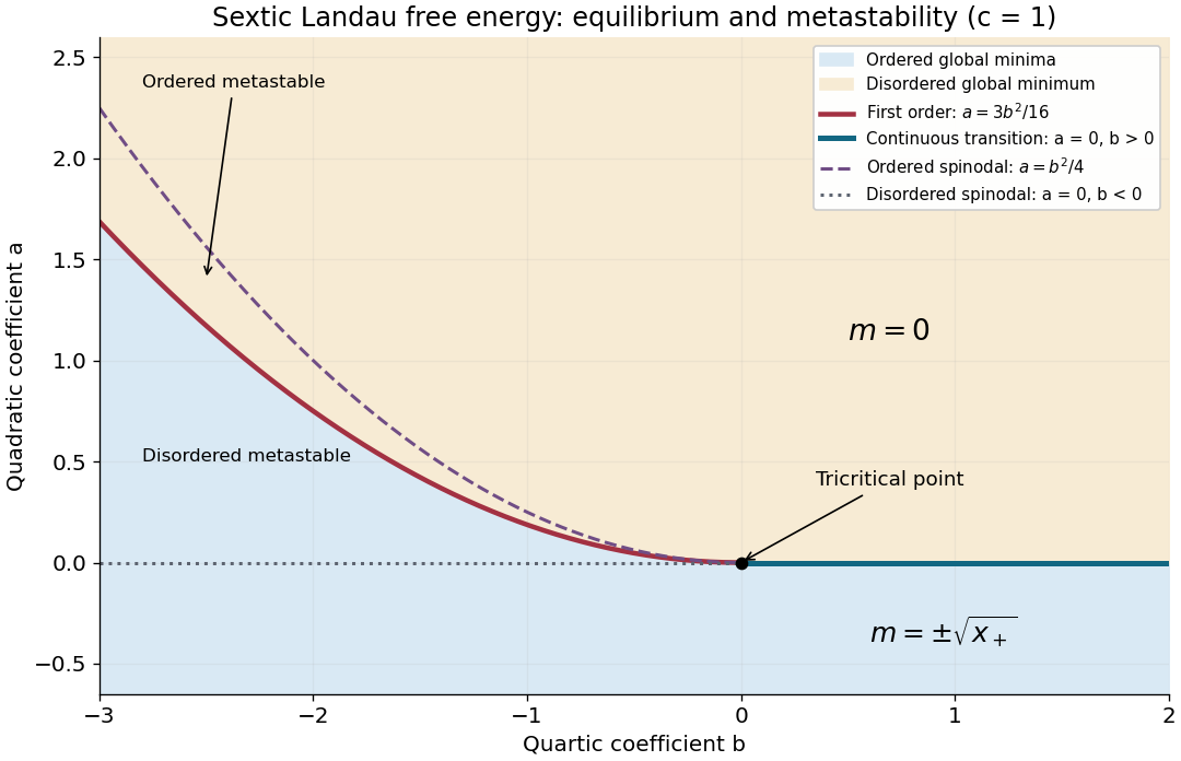
Phase diagram of the sextic Landau free energy, including coexistence, spinodals and the tricritical point
. Details. 
Write , , at fixed , and define the critical exponent by on the ordered side. For fixed and small negative , the stationary equation gives . ConsequentlyAt the tricritical point approached along the tuned path , the stationary equation instead gives , soFor fixed , the transition occurs before reaches zero and the magnetization jumps; it is not a second-order transition and has no vanishing-order-parameter exponent of this form. A path that does not keep the quartic coefficient tuned to zero generally crosses over to the ordinary result.
Take and hold fixed. The heat capacity comes from the minimized free energy, , with any smooth background added separately. For and ,Above , and the polynomial contributes zero. There is a finite jump, rather than a divergence: the conventional ordinary mean-field critical exponents areThe upper branch has zero order-parameter contribution; a finite regular heat capacity has exponent zero.
Along the tuned tricritical path , the ordered minimum givesUpper-side qualification: the vanishing disordered-side heat-capacity amplitude in Landau theory matters here: for and , the minimizing solution is still exactly , so this saddle-point polynomial gives and . A zero function cannot determine a nonzero-amplitude power-law exponent. For example, adding the allowed smooth background , with , leaves the entire phase diagram unchanged but makes the upper-side heat capacity exactly , not a divergence.
One convention assigns the tricritical scaling exponent to both sides, writing with at this mean-field approximation saddle. If the source's literal is meant to have a nonzero leading coefficient, the given polynomial establishes no upper-side tricritical singular exponent; with a nonzero smooth background its leading upper-side exponent is zero. A nonzero upper-side singularity requires fluctuation information beyond this minimization. This distinction prevents claiming an upper-side divergence that the displayed Landau free energy does not produce.
Articles by others on the same topic
There are currently no matching articles.