Functional programming, design and analysis of algorithms (A10097W1)

Source release: Oxford examination archive, member 2018/T/a10097w1.pdf. The cover dates this paper to 18 June 2019; the archive member's directory is misleading. The solutions cover every option. In the code, different definitions offered in different parts are alternatives, and the Haskell Prelude operations have their usual meanings unless redefined locally.

Table of contents
- 1 Functional programming, design and analysis of algorithms
  - a 1
    - Solution a
  - b 1
    - Solution b
  - c 1
    - Solution c
  - d 1
    - Solution d
  - e 1
    - Solution e
  - f 1
    - Solution f
  - g 1
    - Solution g
- 2 Functional programming, design and analysis of algorithms
  - a 2
    - Solution a
  - b 2
    - Solution b
  - c 2
    - Solution c
  - d 2
    - Solution d
  - e 2
    - Solution e
  - f 2
    - Solution f
  - g 2
    - Solution g
- 3 Functional programming, design and analysis of algorithms
  - a 3
    - Solution a
  - b 3
    - Solution b
  - c 3
    - Solution c
  - d 3
    - Solution d
  - e 3
    - Solution e
  - f 3
    - Solution f
- 4 Functional programming, design and analysis of algorithms
  - a 4
    - Solution a
  - b 4
    - Solution b
  - c 4
    - Solution c
  - d 4
    - Solution d
  - e 4
    - Solution e
  - f 4
    - Solution f
  - g 4
    - Solution g
- 5 Functional programming, design and analysis of algorithms
  - a 5
    - Solution a
  - b 5
    - Solution b
  - c 5
    - Solution c
  - d 5
    - i d
      - Solution i
    - ii d
      - Solution ii
    - iii d
      - Solution iii
- 6 Functional programming, design and analysis of algorithms
  - a 6
    - i a
      - Solution i
    - ii a
      - Solution ii
    - iii a
      - Solution iii
  - b 6
    - Solution b
  - c 6
    - Solution c
  - d 6
    - i d
      - Solution i
    - ii d
      - Solution ii
- 7 Functional programming, design and analysis of algorithms
  - a 7
    - Solution a
  - b 7
    - i b
      - Solution i
    - ii b
      - Solution ii
    - iii b
      - Solution iii
  - c 7
    - i c
      - Solution i
    - ii c
      - Solution ii
- 8 Functional programming, design and analysis of algorithms
  - a 8
    - Solution a
  - b 8
    - Solution b
  - c 8
    - i c
      - Solution i
    - ii c
      - Solution ii
  - d 8
    - i d
      - Solution i
    - ii d
      - Solution ii

1

 0  0

a

 0  0

Solution

 0  0

The right fold replaces the two list constructors by its two arguments; the left fold instead updates an accumulator while traversing the list.

foldr :: (a -> b -> b) -> b -> [a] -> b
foldr c z []     = z
foldr c z (x:xs) = c x (foldr c z xs)

foldl :: (b -> a -> b) -> b -> [a] -> b
foldl s a []     = a
foldl s a (x:xs) = foldl s (s a x) xs

Thus foldr is the natural list fold: it preserves the constructor arrangement while replacing [] by z and (:) by c. In particular, foldr (:) [] = id. More generally, the fold factorisation criterion says that the defining equations characterize the corresponding structural recursion. Association and lazy evaluation are separate: the accumulator in this definition of left fold is not automatically evaluated at each step.^[ref]

b

 0  0

Solution

 0  0

For every accumulator

a

, pattern matching makes foldl s a undefined the bottom value. Now use structural induction on a finite list prefix ending in the bottom value. The induction step is foldl s a (x:ps) = foldl s (s a x) ps; the induction hypothesis applies to every accumulator, including s a x. Consequently every such finite approximation has result

⊥

An infinite lazy list is the limit of its finite prefixes, each interpreted as a finite approximation of a lazy list. Definable Haskell operations are Scott continuous maps, so the result on the infinite lazy list is the supremum of the results on these approximations. Every result is

⊥

, hence foldl s a xs = undefined on every infinite input spine, irrespective of whether s would inspect the accumulator.

For a concrete separation, choose s = (&&), a = True, and xs = False : repeat True. The left fold is

⊥

, whereas the right fold returns False after observing the first element: False && r does not demand r. It is reaching the end of the input spine, rather than strictness of the combining operation, that prevents this left fold from returning.

c

 0  0

Solution

 0  0

Over integers, choose s = c = (+) and a = b = 0. The left fold and right fold both compute the sum of a finite list.

d

 0  0

Solution

 0  0

Over integers, choose s = (-), c = flip (-), and a = b = 0. The left fold and right fold both compute the negative of the sum of a finite list. The combining functions differ: s 1 2 = -1, whereas c 1 2 = 1.

e

 0  0

Solution

 0  0

Let

F = foldl (⊖) 0

, using the specified operation

u ⊖ v = v - u

. Direct evaluation gives

F ([]) = 0

F ([0]) = 0

F ([1]) = 1

, and

F ([1, 0]) = - 1

Suppose

F = foldr c b

with the same integer result type. The empty list forces

b = 0

. The two singleton calculations force

c 00 = 0

and

c 10 = 1

. But then

F ([1, 0]) = c 1 (c 00) = c 10 = 1,

(1)

contrary to

F ([1, 0]) = - 1

. No such c,b exist. This is the information restriction in the fold factorisation criterion: equal folded tails must remain indistinguishable after the same head is attached. A larger, function-valued result type can retain the missing information, as the continuation representation of a left fold does below.

f

 0  0

Solution

 0  0

Assign

y : u

and

x : v

. The application s y x forces

s : u \to v \to w

for a fresh type

w

; applying f to that result forces

f : w \to r

. No further equations identify these four type variables. The principal type is therefore

k :: (u -> v -> w) -> v -> (w -> r) -> u -> r
k s x f y = f (s y x)

Every compatible typing is an instance of this one, because type inference imposed precisely the two application constraints and no class constraints.

g

 0  0

Solution

 0  0

Fix s and put

R (x s, a) = foldr (k s) id x s a

. The right fold equations give

R ([], a) = a, R (x : x s, a) = R (x s, s a x) .

(1)

These are exactly the left fold equations. Structural induction, with the induction hypothesis quantified over all accumulators, proves equality on finite terminating lists.

To include the other input spines, first observe that both applied expressions give

⊥

on an undefined spine. The same induction proves equality on every finite prefix ending in

⊥

: the step k s x f a demands the continuation f when its result is demanded. Finally use that the two applied operations are Scott continuous maps, taking the limit over prefixes interpreted as a finite approximation of a lazy list. This covers infinite spines, on which both applied expressions are

⊥

, and proves the identity for all lists under the stated Haskell semantics. The intermediate right fold builds an accumulator-transforming function; it does not provide a terminating left fold of an infinite list.

2

 0  0

a

 0  0

Solution

 0  0

Include nonpositive counts and exhausted input explicitly:

take :: Int -> [a] -> [a]
take n _      | n <= 0 = []
take _ []             = []
take n (x:xs)         = x : take (n-1) xs

drop :: Int -> [a] -> [a]
drop n xs     | n <= 0 = xs
drop _ []             = []
drop n (_:xs)         = drop (n-1) xs

The tests on the count precede inspection of the input list. Thus take 0 undefined = [], while drop 0 undefined = undefined, exactly as these list prefix and list suffix operations require. No element value is inspected merely to traverse the spine.^[ref]

b

 0  0

Solution

 0  0

A shared recursion computes both components:

split :: Int -> [a] -> ([a],[a])
split n xs | n <= 0 = ([],xs)
split _ []         = ([],[])
split n (x:xs)     = (x:ys,zs)
  where (ys,zs) = split (n-1) xs

For a defined count and a spine with

m

available constructors before termination, each of take and drop makes

min (max (n, 0), m)

recursive calls, whereas split makes that many once. The number of recursive calls is halved. The irrefutable pattern in the local pair binding also avoids evaluating the recursive pair merely to expose the first output element.

On proper lazy lists this has the intended two component values. There is a small bottom value distinction outside that domain: the displayed single-pass definition must inspect a positive-count input spine before returning its outer pair, whereas the literal expression (take n xs, drop n xs) exposes the pair constructor even if xs is undefined. The algorithmic answer concerns the two components and the stated call count; it need not silently claim equality under a test that observes this outer constructor alone.

c

 0  0

Solution

 0  0

For the paper's leaf-labelled binary tree, the combining operation receives the results of the two subtrees, and the other argument handles a leaf:

foldTree :: (a -> b) -> (b -> b -> b) -> Tree a -> b
foldTree f g (One x)   = f x
foldTree f g (Two l r) = g (foldTree f g l) (foldTree f g r)

Its constructor equation is foldTree One Two = id. More generally, a function h satisfying h (One x) = f x and h (Two l r) = g (h l) (h r) equals foldTree f g on finite trees, by structural induction. This is the tree fold specialized to a datatype with labels only at leaves, rather than at internal nodes.

d

 0  0

Solution

 0  0

Both versions preserve left-to-right leaf order:

flatten :: Tree a -> [a]
flatten (One x)   = [x]
flatten (Two l r) = flatten l ++ flatten r

flattenFold :: Tree a -> [a]
flattenFold = foldTree (\x -> [x]) (++)

The tree fold replaces each leaf by a singleton list and each internal node by list concatenation. The defining equations of flattenFold are consequently those of flatten, proving their equality by structural induction.

e

 0  0

Solution

 0  0

Let

n

be the number of leaves; the total number of nodes is

2 n - 1

. List concatenation copies its left operand. For a tree whose left subtree contains

n - 1

leaves at each successive internal node, these copied lengths are

1, 2, \dots, n - 1

. Their sum is

n (n - 1) /2

, so the worst-case running time is $Θ (n^{2})$ .

A difference list representation avoids copying prefixes:

flattenFast :: Tree a -> [a]
flattenFast t = go t []
  where
    go (One x)   acc = x:acc
    go (Two l r) acc = go l (go r acc)

The recursion invariant is go t acc = flatten t ++ acc. The leaf case is immediate; the internal-node case uses associativity of list concatenation. Each node is visited once and each leaf contributes one output constructor, giving $Θ (n)$ running time when the result is fully consumed. This is linear flattening of a binary tree and does not assume balance.

f

 0  0

Solution

 0  0

The necessary domain is a finite, nonempty list: the datatype has no representation of an empty leaf sequence, and the supplied size-based balance condition does not specify an infinite-size construction.

build :: [a] -> Tree a
build []  = error "build: empty input"
build [x] = One x
build xs  = Two (build ys) (build zs)
  where
    (ys,zs) = split (length xs `div` 2) xs

For length

n \geq 2

, the two nonempty pieces have

⌊ n /2 ⌋

and

⌈ n /2 ⌉

elements. Their sizes differ by at most one, and both are shorter than the input. Induction therefore proves termination and the required leaf-balanced binary tree property at every node. The same induction, using ys ++ zs = xs, proves flatten (build xs) = xs. This straightforward implementation takes

O (n lo g n)

running time; computing the length repeatedly is acceptable here because no faster construction was requested.

g

 0  0

Solution

 0  0

Use the input list as the seed of the tree unfold:

buildUnfold :: [a] -> Tree a
buildUnfold = unfold step
  where
    step []  = error "build: empty input"
    step [x] = Left x
    step xs  = Right (split (length xs `div` 2) xs)

On a singleton seed, unfold produces the same leaf as build; on a longer finite seed, it recursively builds the same two pieces. Induction on input length proves buildUnfold = build on finite nonempty inputs. The empty-input qualification remains essential: a tree unfold cannot supply a missing empty-tree constructor.

3

 0  0

a

 0  0

Solution

 0  0

Use coordinates with row and column in

{0, 1, 2}

type Place  = (Int,Int)
type Places = [Place]
type Board  = (Places,Places,Places)
data Player = O | X deriving (Eq,Ord,Show)

The components of Board record the positions occupied by O, occupied by X, and still empty, respectively. On a nonterminal legal board, equal occupied counts mean O moves next; one extra O means X moves next.

The type synonym does not enforce the representation invariant: coordinates are in range; each component has no duplicates; the three represented sets form a set partition of the nine positions; and the occupied counts differ as just described. Both players cannot have won. A winning O board has one extra O, and a winning X board has equal counts. More fundamentally, a legal tic-tac-toe state has a legal alternating history that stops at the first win: satisfying a type alone never licenses continuing an already completed game.

b

 0  0

Solution

 0  0

The empty occupancy sets leave all nine coordinates available:

empty :: Board
empty = ([],[],[(r,c) | r <- [0..2], c <- [0..2]])

This board satisfies the representation invariant and gives O the next move.

c

 0  0

Solution

 0  0

Assume the board satisfies the representation invariant. Reject completed boards and occupied or out-of-range coordinates; testing membership in the empty component covers both coordinate failures.

finished :: Board -> Bool
finished (os,xs,es) = won os || won xs || null es

play :: Board -> Place -> Board
play b@(os,xs,es) q
  | finished b     = error "play: completed game"
  | q `notElem` es = error "play: unavailable place"
  | length os == length xs = (q:os,xs,rest)
  | otherwise             = (os,q:xs,rest)
  where rest = filter (/=q) es

Here won is defined in part d. Moving one available coordinate into the appropriate occupied component preserves the set partition and the alternating-count rule. Checking completion first preserves the no-moves-after-a-win invariant.

d

 0  0

Solution

 0  0

Construct each possible winning line, then test whether one is contained in the player's occupancy set:

winningLines :: [Places]
winningLines =
  [[(r,c) | c <- [0..2]] | r <- [0..2]] ++
  [[(r,c) | r <- [0..2]] | c <- [0..2]] ++
  [[(i,i) | i <- [0..2]], [(i,2-i) | i <- [0..2]]]

won :: Places -> Bool
won ps = any (\line -> all (`elem` ps) line) winningLines

The list comprehension generates three rows, three columns and two diagonals. Each has exactly three coordinates; therefore all holds precisely when every coordinate of that line is occupied by this player. Taking any over the eight lines proves the win test correct.

e

 0  0

Solution

 0  0

Record the outcome at the first completed board and otherwise branch over every available move:

data Outcome = Winner Player | Draw deriving (Eq,Ord,Show)

finals :: Board -> [(Board,Outcome)]
finals b@(os,xs,es)
  | won os    = [(b,Winner O)]
  | won xs    = [(b,Winner X)]
  | null es   = [(b,Draw)]
  | otherwise = concatMap (\q -> finals (play b q)) es

The recursion terminates because each recursive call decreases the number of empty positions by one. For correctness, induct on that number. A completed board contributes exactly its own outcome. Otherwise every legal continuation has a unique first available move, and the induction hypothesis covers exactly all completions after that move. List concatenation collects these branches without extending completed games. Repeated final positions are allowed here because the computation deliberately explores every legal move sequence.

f

 0  0

Solution

 0  0

Different move orders can lead to the same position, and the two occupancy lists also retain irrelevant insertion order. Thus this search tree repeatedly solves the same remaining game. For example, swapping the order of two O moves while leaving the intervening X moves legal can reach the same occupied sets.

Canonicalize each state by sorted occupancy sets, or by two bitboards, and apply memoization or a visited-state set. Expand each canonical position once, stopping at terminal states, and collect terminal positions in a set. There are at most

3^{9}

cell assignments, many of which are illegal; this is much smaller than a tree of move permutations. Store positions, not histories, when the requested output is distinct final positions. Board rotations and reflections can reduce work further if handled as an additional equivalence: if the output must retain every oriented board, reconstruct those distinct orientations rather than silently returning one representative per symmetry class.

4

 0  0

a

 0  0

Solution

 0  0

For proper lazy lists, the generic condition is a finite first list, or an empty second list. A finite first list reaches its terminating constructor, after which list concatenation exposes the second one. An infinite first list never yields control to the second; it therefore cannot deliver occurrences originating there unless there are none. This concerns input occurrences, rather than an accidental overlap of the two inputs' value sets.

A first spine ending in the bottom value also prevents access to the second list. Such inputs require the partial-input qualification in part c; a visible prefix is different from a terminating finite list.

b

 0  0

Solution

 0  0

Swap roles after emitting one element:

interleave :: [a] -> [a] -> [a]
interleave []     ys = ys
interleave (x:xs) ys = x : interleave ys xs

While both lists are nonempty, the function alternates between them. Their

j

-th input occurrences appear after at most

2 j + 2

output steps, counting positions from zero; once either list ends, the other is returned directly. Every output constructor comes from one input constructor, and every input occurrence is eventually selected. This proves fair enumeration and productivity on the two proper lazy lists, including two infinite ones.

c

 0  0

Solution

 0  0

No universally correct sequential Haskell implementation has that guarantee for partial lists. Compare undefined paired with [v], and [v] paired with undefined, where the element type is arbitrary. A generic program cannot fabricate v; it must eventually inspect an input spine to obtain it. Whichever input it first demands can be chosen to be the undefined one, blocking access to the available element in the other input.

In particular, the implementation in part b can emit a defined prefix and then block when alternation reaches an undefined tail. Lazy evaluation postpones demands; it cannot recognize that a demanded computation will never finish. The result is the partial-list interleaving obstruction, not an objection to fairness under the proper-input hypothesis. Additional concurrent primitives would change the computational model.^[ref]

d

 0  0

Solution

 0  0

Use diagonal merging of lazy lists: introduce one new row each round, and advance every active row once. Each round contains finitely many active rows, even when the outer list is infinite.

fairConcat :: [[a]] -> [a]
fairConcat = concat . levels []
  where
    levels [] [] = []
    levels active pending =
      let (new,rest) = case pending of
            []     -> ([],[])
            r:rs   -> ([r],rs)
          live = [r | r@(_:_) <- active ++ new]
      in map head live : levels (map tail live) rest

Number rows and positions within each row from zero. An occurrence at

(i, j)

is emitted in round $i + j$ : its row enters in round

i

and advances once per subsequent round. All earlier rounds and each round's output are finite, so every required occurrence appears after finite work. live discards only empty rows, and head emits only existing entries; no new value is invented.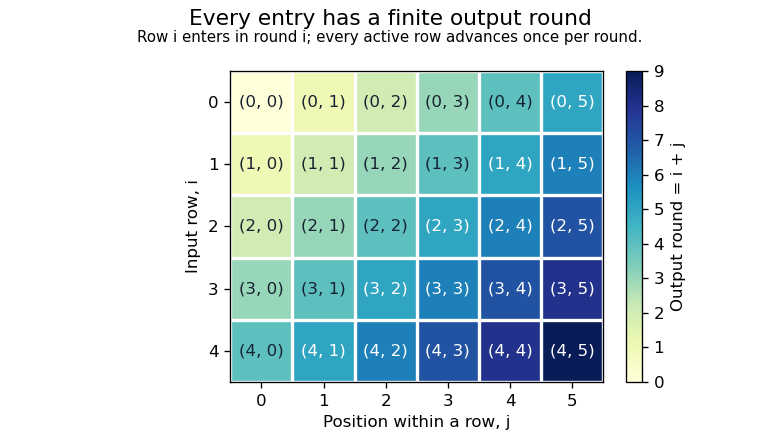

Figure 1.
Diagonal merging of lazy lists visits every finite row-position pair after finitely many rounds
. **Details**.

Simply nesting interleave is unsafe here: foldr interleave [] ([1,2] : repeat []) emits 1 and then demands an undefined merge of the infinitely many empty rows before it can emit 2. The finite-round construction avoids that starvation. There is still an unavoidable termination qualification: after the last actual output, infinitely many empty pending rows cannot be certified empty in finite work. The result can then have an undefined tail instead of a terminating []. Every required occurrence has nevertheless appeared; no generic algorithm can promise a proper completed output in that exceptional situation, by the absence-detection obstruction for infinite lists.

e

 0  0

Solution

 0  0

The ordinary list comprehension exhausts the inner list before advancing the outer one. Therefore it enumerates every argument pair when ys is finite, or when xs has at most one element. If ys is infinite and xs has two or more elements, it stays with the first outer element forever and misses every pair with a later outer occurrence. Applying a constant f might hide missing pairs as duplicate values; it does not make the enumeration fair.

An empty-result caveat remains when ys = [] and xs is infinite: the literal comprehension traverses infinitely many empty rows and does not return a terminating empty list. Its occurrence requirement is vacuous, but its productivity as an empty-result computation fails. An explicit empty-input test avoids that particular failure.

f

 0  0

Solution

 0  0

Merge the rows with fairConcat, retaining explicit empty-input cases:

fairPair :: (a -> b -> c) -> [a] -> [b] -> [c]
fairPair _ [] _  = []
fairPair _ _  [] = []
fairPair f xs ys = fairConcat [[f x y | y <- ys] | x <- xs]

For nonempty proper lazy lists, the occurrence f (xs!!i) (ys!!j) belongs to row

i

, position

j

, so the proof in part d puts it in round

i + j

. This supplies every pair after finite work, even when both input lists are infinite. The guards also return [] for either empty factor without traversing infinitely many empty rows.

g

 0  0

Solution

 0  0

For a finite outer list of proper lazy lists, use the fair binary product from part f:

cp :: [[a]] -> [[a]]
cp []       = [[]]
cp (xs:xss) = fairPair (:) xs (cp xss)

The empty family has one selection, the empty selection. For a nonempty finite family, each selection consists uniquely of one first-factor occurrence followed by a selection from the remaining factors. Induction on the number of factors, together with the fairness of fairPair, proves that every such selection is produced and no invalid selection is introduced. Infinite factors are allowed: in particular, the three-factor example is enumerated fairly. If any factor is empty, the finite-family computation returns the empty product.

The printed hypothesis also permits an infinite outer proper lazy list. No function can satisfy the full enumeration requirement for all such inputs. Take repeat [0,1]. Its mathematical Cartesian product contains every infinite binary sequence and is uncountable. If a result list enumerated these sequences as

z_{0}, z_{1}, \dots

, the binary sequence

b

with

b_{i} = 1 - z_{i} (i)

would differ from the

i

-th listed sequence at position

i

, contradicting completeness. This is an uncountability obstruction to enumerating infinite Cartesian products. The finite-outer qualification is a necessary repair to the specification, not a restriction imposed for convenience by the code.

5

 0  0

a

 0  0

Solution

 0  0

A divide-and-conquer algorithm handles a small input directly; otherwise it divides the input into smaller instances, recursively solves them, and combines their answers. With

a

equally sized subproblems of size approximately

n / b

and nonrecursive work

f (n)

, its recurrence relation has the form

T (n) = a T (n / b) + f (n)

, with constant-size base cases,

a \geq 1

and

b > 1

Write

p = lo g_{b} a

. The basic master theorem gives the following cases, with a fixed

ε > 0

If $f (n) = O (n^{p - ε})$ , then $T (n) = Θ (n^{p})$ .
If $f (n) = Θ (n^{p})$ , then $T (n) = Θ (n^{p} lo g n)$ .
If $f (n) = Ω (n^{p + ε})$ and the regularity condition $a f (n / b) \leq c f (n)$ holds eventually for some $c < 1$ , then $T (n) = Θ (f (n))$ .

For the common extended middle case,

f (n) = Θ (n^{p} lo g^{k} n)

with fixed

k \geq 0

gives

T (n) = Θ (n^{p} lo g^{k + 1} n)

. A recursion tree explains the three cases: work is dominated by its leaves, spread across comparable levels, or dominated by its top levels. The regularity condition in the last case is part of the theorem, not an optional simplification.

b

 0  0

Solution

 0  0

For an ascending sorted array, maintain a candidate interval

[ℓ, r]

initially containing every index. Compare the target with the middle entry at

m = ⌊(ℓ + r) /2 ⌋

. Equality returns

m

; if the target is smaller, replace

r

m - 1

; if larger, replace

ℓ

m + 1

. An empty interval reports absence.

The loop invariant is that any target occurrence still possible lies inside the candidate interval. Sortedness justifies discarding the appropriate half after each unequal comparison. The interval length decreases to at most half its previous length, establishing termination and correctness. After

t

unsuccessful comparisons there are at most

n / 2^{t}

candidates, so at most

⌊ lo g_{2} n ⌋ + 1

comparisons suffice for

n \geq 1

. Each iteration uses constant work on a random-access array. Thus binary search takes $O (lo g (n + 1))$ running time, conventionally written

O (lo g n)

for nontrivial input sizes. Empty input is handled in constant time.

c

 0  0

Solution

 0  0

Assume ascending sorted arrays; descending storage can be accessed in reverse index order without copying. Among

2 n

entries, the requested rank is $k = n + 1$ in ascending order, not

n

. Repeated values occupy repeated ranks.

Choose

i

entries from the first array and

j = k - i

from the second, using their prefixes. The feasible range is

max (0, k - n) \leq i \leq min (n, k)

. Write

A_{L} = A [i]

A_{R} = A [i + 1]

, and similarly

B_{L}, B_{R}

j

, with missing left endpoints replaced by

- \infty

and missing right endpoints by

+ \infty

. These are conceptual sentinels, not extra stored entries.

Use binary search over the feasible values of

i

If $A_{L} > B_{R}$ , there are too many entries from $A$ on the left; decrease the upper bound to $i - 1$ .
If $B_{L} > A_{R}$ , there are too few entries from $A$ on the left; increase the lower bound to $i + 1$ .
Otherwise return $max (A_{L}, B_{L})$ .

For correctness, in the last case every left entry is no greater than every right entry, and exactly

k

entries lie on the left. Their maximum is therefore the

k

-th smallest entry. The failed inequalities are monotone in the searched index: increasing

i

raises the

A

boundary and decreases the

B

boundary, so it cannot repair

A_{L} > B_{R}

; the other case is symmetric. A partition of the first

k

entries of a merged ordering supplies an admissible solution, including ties. Each step halves an interval with at most

n + 1

choices, giving $O (lo g (n + 1))$ running time and $O (1)$ auxiliary space. This is a two-sorted-array order statistic without constructing the merged array.

d

 0  0

i

 0  0

Solution

 0  0

If coordinate

j

is not an essential variable of a function, changing that coordinate alone never changes the output, for any values of the other coordinates. Take two inputs with the same

i

-th coordinate. Change their other coordinates one at a time to transform the first input into the second. Every such change is inessential, so all intermediate outputs are equal.

Define

f_{i} (t) = f (1, \dots, 1, t, 1, \dots, 1)

, with

t

in position

i

. The preceding argument gives $f (x_{1}, \dots, x_{n}) = f_{i} (x_{i})$ . Since

i

is essential,

f_{i}

is nonconstant. The conclusion depends on the full “for every context” negation of essentiality, not merely on testing a coordinate at one selected input.

ii

 0  0

Solution

 0  0

n = 1

, return its sole index without a query. Otherwise first evaluate

f (t, t, \dots, t)

for

t = 1, \dots, d

until two different outputs are found. Part i says these outputs are precisely

f_{i} (t)

, so two values

a, b

with

f_{i} (a) \neq = f_{i} (b)

must exist. This uses at most

d

calls to the function-evaluation oracle.

Maintain a candidate index set

S

, initially all indices. Split

S

into two nearly equal pieces and choose one,

H

. Query the input that is

b

H

and

a

everywhere else. Its output equals

f_{i} (b)

exactly when

i \in H

, and otherwise equals

f_{i} (a)

. Retain the indicated half and repeat until one index remains.

The loop invariant is

i \in S

, and the witness outputs keep each test unambiguous. There are at most

⌈ lo g_{2} n ⌉

splitting queries. The total is at most $d + ⌈ lo g_{2} n ⌉$ evaluations, which is

O (d lo g n)

for

n \geq 2

, and in fact a stronger additive bound. Only oracle calls are being counted; explicitly constructing each query vector can require

O (n)

ordinary work. This is identification of a unique essential variable.

iii

 0  0

Solution

 0  0

Restrict the unknown function to the

n

possibilities

f^{(i)} (x) = 1

x_{i} = 1

, and

2

otherwise. Each has exactly one essential variable, even if the allowed alphabet has more than two values. Every oracle answer in this restricted family is one bit.

A correct adaptive deterministic algorithm must distinguish all

n

possibilities. A binary decision tree of depth

q

has at most

2^{q}

leaves, so

2^{q} \geq n

. Therefore $q \geq ⌈ lo g_{2} n ⌉ = Ω (lo g n)$ . Restricting the answer family is essential to the argument: unrestricted integer-valued answers need not have binary branching. Combined with part ii, this gives optimal logarithmic query complexity for fixed

d

6

 0  0

a

 0  0

i

 0  0

Solution

 0  0

Store a complete binary tree in a one-indexed array

A [1.. n]

, level by level. Index

i

has parent in a rooted tree

⌊ i /2 ⌋

for

i > 1

and possible children in a rooted tree

2 i

and

2 i + 1

, present only when their indices are at most

n

. The max-heap condition is

A [⌊ i /2 ⌋] \geq A [i]

for every

i > 1

Following these inequalities from the root of a tree to any entry proves that $A [1]$ is a maximum. The heap order does not sort siblings or unrelated branches. The complete binary tree has height

⌊ lo g_{2} n ⌋

, which bounds how far any single repair can travel. Store the current heap size separately from the array's capacity.

ii

 0  0

Solution

 0  0

Assume the subtrees rooted at the children in a rooted tree of

i

already obey the max-heap condition. Compare

A [i]

with each present child and choose an index of the largest of these at most three keys. If that index is

i

, stop. Otherwise exchange the two keys, continue at the chosen child, and repeat. This is sift down, with the inequality reversed from a minimum-oriented binary heap.

The exchange repairs the old root position because its new key dominates both child roots; only the subtree receiving the displaced key can still be defective. This recursion invariant proves correctness. Each exchange descends one level and costs constant work, so the worst-case running time is $O (h)$ for subtree height $h$ , hence $O (lo g n)$ . A small key at the root of a suitably ordered heap must descend to a leaf, so the logarithmic worst-case bound is attained.

iii

 0  0

Solution

 0  0

Leaves already obey the heap order. Process indices

⌊ n /2 ⌋, ⌊ n /2 ⌋ - 1, \dots, 1

, calling the preceding repair at each. When an index is processed, its descendants have already been processed, so the repair's precondition holds. The resulting array is a max-heap.

The bound obtained by charging

O (lo g n)

to every call is unnecessarily large. The number of nodes with height at least

h

is at most

⌊ n / 2^{h} ⌋

. Therefore

\sum_{v} (1 + height (v)) \leq n + \sum_{h \geq 1} ⌊ n / 2^{h} ⌋ < 2 n .

(1)

The total repair work is thus $O (n)$ , and the loop itself has a linear number of iterations, giving $Θ (n)$ for this bottom-up heap construction. Most nodes are near the leaves and require little repair.

b

 0  0

Solution

 0  0

A maximum priority queue stores keyed entries and supports insertion, inspection and removal of an entry with greatest key, and key increases. A max-heap gives the following running times, with the size/capacity cost of the backing array accounted for separately:

maximum: return the root key in $O (1)$ time.
insert: append at the next available leaf, then use sift up until the heap order holds, in $O (lo g n)$ time.
extractMaximum: save the root, replace it by the last entry, reduce the size, and use sift down, in $O (lo g n)$ time.
increaseKey(i,k): reject $k < A [i]$ ; otherwise set the new key and use sift up, in $O (lo g n)$ time.
isEmpty and size: inspect the stored size in $O (1)$ time; construct a queue from $n$ keys by bottom-up heap construction in $Θ (n)$ time.

Empty-queue inspections and removals need an explicit failure result. The index argument to increaseKey must identify the entry's current location: if callers use item handles, update their location records during swaps.

c

 0  0

Solution

 0  0

Given the target's current heap index

i

, remove it as follows. If

i = n

, discard the last entry. Otherwise replace

A [i]

A [n]

and reduce

n

by one. If the replacement is larger than its parent in a rooted tree, use sift up; otherwise use the maximum-oriented sift down from

i

Only comparisons incident to the replacement can initially violate the heap order. If it exceeds its parent, it also dominates the old children because the old key dominated those children and was no larger than the parent; an upward repair suffices. Otherwise the upward comparison is valid and only a downward repair can be needed. Thus removal takes $O (lo g n)$ worst-case time after the location is known. Searching an unindexed heap for an arbitrary specified key can instead require

Θ (n)

time; the logarithmic bound does not include such a search.

d

 0  0

i

 0  0

Solution

 0  0

Only arrange switches towards A. For every vertex

u

, compute its degree

de g (u)

and the current number

c (u)

of neighbours preferring A. Put the B vertices in a max-heap with key

q (u) = 2 c (u) - de g (u)

. Maintain each vertex's current heap array index during exchanges.

While the queue is nonempty and its maximum key is positive, extract that vertex

u

, show it its neighbours' preferences, append

u

to the answer sequence, and set its preference to A. For every neighbour

v

still preferring B, increase

c (v)

by one and use increaseKey to increase its heap key by two. Stop when every remaining key is nonpositive.

A positive key means precisely a strict majority of A neighbours, so every listed move is legal. Degrees never change; A neighbours never revert in this chosen sequence. An isolated B vertex has key zero and cannot be converted. Initialization costs

O (∣ V ∣ + ∣ E ∣)

, there are at most

∣ V ∣

extractions, and each edge causes at most two neighbour inspections and at most a constant number of key updates. The required bound is therefore $O ((∣ V ∣ + ∣ E ∣) lo g (∣ V ∣ + 1))$ . A simple work queue of newly eligible vertices can even implement the same monotone threshold activation in

O (∣ V ∣ + ∣ E ∣)

time, since a vertex needs to be enqueued only once.

ii

 0  0

Solution

 0  0

Let

C

be the final A set produced by the algorithm. It contains the initial A set, and every vertex outside

C

has at most half its neighbours in

C

: otherwise its final key would still be positive. Thus

C

is closed under the activation rule.

Now consider any legal sequence, including sequences which change some A preferences back to B. We prove by induction that its current A set is always a subset of

C

. This is true initially. A switch to B preserves the inclusion. If a vertex outside

C

were to switch to A, its A neighbours would all lie in

C

, so their number could not exceed half its degree. Such a switch is forbidden. A switch inside

C

also preserves the inclusion.

Consequently every attainable final A set has size at most

∣ C ∣

. The algorithm supplies a legal sequence attaining

C

itself, so its sequence is optimal. This closure dominance for asynchronous threshold switching proves more than a local-greedy claim: temporary losses of A vertices cannot unlock an additional vertex outside the activation closure.

7

 0  0

a

 0  0

Solution

 0  0

Use unit-cost insertion, deletion and substitution of one symbol. Their minimum total cost is the edit distance. Let

D [i, j]

be the edit distance between the first

i

symbols of the first sequence and the first

j

of the second. Initialize

D [i, 0] = i

and

D [0, j] = j

. For

i, j > 0

compute

D [i, j] = min {D [i - 1, j] + 1, D [i, j - 1] + 1, D [i - 1, j - 1] + [x_{i} \neq = y_{j}]} .

(1)

The cases delete the final source symbol, insert the final target symbol, or align the two final symbols, paying one for substitution and zero for a match. Every optimal alignment ends in one of these cases, and each case extends a valid shorter alignment. Induction on

i + j

proves the dynamic programming recurrence correct.

Fill rows or columns in increasing order so every dependency is already available. There are

(m + 1) (n + 1)

entries with constant work per interior entry: $O (mn)$ running time for nonempty sequences, or

O ((m + 1) (n + 1))

including the boundary cases. The full table has space complexity

O (mn)

; two rows give

O (n)

auxiliary space when only the distance is wanted. Predecessor choices in the full table recover an optimal edit sequence.

b

 0  0

i

 0  0

Solution

 0  0

For nonnegative integer amount

v

, let

M [t]

be the minimum number of coins making amount

t

. Set

M [0] = 0

and compute, in increasing order of

t

M [t] = 1 + min_{i : x_{i} \leq t} M [t - x_{i}], 1 \leq t \leq v .

(1)

An empty candidate set has minimum

\infty

. Here denomination

1

ensures that every nonnegative amount is attainable. Removing one coin from an optimal nonempty solution gives a smaller amount, and adding any allowed last coin gives a feasible solution; these two directions prove the recurrence by induction on

t

Return whether $M [v] \leq k$ . This solves the at-most-

k

decision without needing a separate dimension for

k

. The table for the minimum coin change recurrence takes $O (n v)$ running time and $O (v)$ space complexity. The bound is pseudopolynomial time: the amount, rather than its binary encoding length, appears in it. Amount zero needs zero coins.

ii

 0  0

Solution

 0  0

During the computation in part i, record an index

last [t]

attaining the minimum at every positive amount. Starting with

t = v

, print

x_{last [t]}

and replace

t

t - x_{last [t]}

, continuing until

t = 0

Every step decreases the amount and reduces the table entry by exactly one. The printed denominations therefore sum to

v

and their number is exactly

M [v]

, proving optimality. The total running time is $O (n v + M [v])$ , including the output;

M [v] \leq v

because denomination

1

is available. The predecessor array adds

O (v)

to the space complexity. This is reconstruction from the dynamic programming certificate, not the largest-denomination greedy algorithm, which need not be optimal for arbitrary denominations.