The Paul trap alternates focusing and defocusing electric forces. Their time average along a moving trajectory need not vanish, even when the electric field averages to zero at every fixed point. A spatial gradient makes the fast displacement correlate with the driving electric field; the RF-averaged trapping potential calculates the resulting restoring force.
Wolfgang Paul's lecture describes hyperbolic ring/endcap electrodes, loading by Electron-impact ionization of low-pressure gas, and resonant ejection through an endcap hole into an electron multiplier. Sweeping RF voltage produces an air mass spectrum.[ref]
Electromagnetic traps for charged and neutral particles by Wolfgang Paul. Paul, pp. 608–614, Figs. 6, 11; Columbia scan
Specify the convention before quoting a stability parameter. Choose the ideal, rotationally symmetric electric potentialHere is a static voltage coefficient, is a peak RF voltage coefficient, is the length entering this displayed normalization, is mass, is signed electric charge, and is the drive angular frequency. The coefficient is neither a peak-to-peak voltage nor an RMS voltage. An apparatus's ring-to-cap voltage requires matching its electrode surfaces to this electric potential; electrode radius alone does not define our . The minus sign fixes the RF phase at .
With , Newton's second law gives a Mathieu equation for each Cartesian coordinate :Thus a three-dimensional Paul trap needs simultaneous bounded solutions in all three directions. Changing the sign of reverses and shifts the RF phase by half a cycle; it does not change the ideal infinite-time stability regions. Rescaling the voltage or length convention changes the numerical parameters. Floquet theory determines stability of the full Mathieu equation; the small-parameter approximation below does not establish stability for arbitrary . Bounded mathematical motion can still hit an electrode if its amplitude exceeds the available space.
Write the RF electric field as , where is a real peak-amplitude vector with a common drive phase. Decompose the trajectory into a slow position and fast displacement . Over one short RF cycle, hold fixed. The leading fast equation and solution areThe homogeneous slow part is absorbed into . Expand the electric field to first order in and average, using :The second equality uses zero curl in the quasistatic RF electric field. This derives an effective potential energy, not an extra static electric potential. Its dependence confines either sign of electric charge towards a field-amplitude minimum. Using an RMS field instead would give a coefficient multiplying .
The approximation needs fast displacement small compared with the field's variation length and slow angular frequencies small compared with . In the stated electric quadrupole model, small and of order provide a controlled regime, away from stability boundaries. Add when . For the result isFor the pure RF case, . The square-root condition describes leading local restoring curvature; it is not a substitute for full Mathieu equation stability. Collisions, departures from the ideal electric quadrupole, and a displaced RF null require further analysis.
The slow part of a trapped trajectory in the small-parameter regime of a Paul trap. Its angular frequency is approximately set by the curvature of the RF-averaged trapping potential, including any static electric potential contribution. Paul trap micromotion is superposed on this slow motion.
In the small-parameter regime, the slow coordinate describing Paul trap secular motion approximately obeys a harmonic oscillator equation at angular frequency . Its superposed fast motion is Paul trap micromotion. Substituting the leading fast displacement from the RF-averaged trapping potential gives the displayed expression in our phase convention. A small positional ripple can have substantial velocity, because differentiating it brings down the large angular frequency . Precision spectroscopy must therefore address both Paul trap secular motion and Paul trap micromotion; merely obtaining a bounded trajectory does not eliminate Doppler shifts.
Choose these dimensionless parameters for an original example, with no collisions or damping. They are teaching inputs, not measurements from either lecture. With and slow initial amplitude , the radial equation and its leading approximation areSet and to match the approximate initial conditions. The leading secular angular frequency is . The velocity Verlet method integrates the full RF equation over 80 drive periods; a separate fourth-order Runge-Kutta method checks the computed trajectory. Halving the timestep tests numerical error independently of the averaging error.
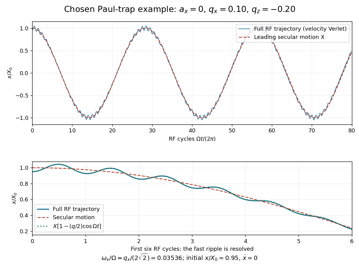
Full RF motion and the leading secular approximation
. Original chosen small-parameter calculation in units of . The lower panel resolves six drive cycles and includes the first micromotion correction. Agreement over this finite interval does not establish a stability diagram or an exact secular frequency. Details.
Using 400, 800, 1600 and 3200 steps per RF period gives successive maximum position differences of approximately , and in units of , consistent with second-order convergence. The finest trajectory differs from the independent classical fourth-order Runge-Kutta method result by at most , whereas differs by as much as . Over a sufficiently long time, the omitted correction to the secular angular frequency produces a growing phase discrepancy even if the numerical trajectory has converged. For the chosen point only, integration of a fundamental solution matrix over one RF period checks that both the radial and axial Floquet multipliers lie on the unit circle, away from its endpoints. This tests simultaneous ideal confinement without extrapolating to larger .
Articles by others on the same topic
There are currently no matching articles.