An ion trap confines an ion using electromagnetic fields, allowing repeated interrogation of the same particle. The name also covers related traps for an Electron. A Paul trap uses an oscillating electric quadrupole field; a Penning trap combines a static electric quadrupole field with a static magnetic field. Confinement creates time to measure an energy level, frequency or magnetic dipole moment; it does not itself cool the particle or identify its internal quantum state.
The obstacle is Earnshaw's theorem. In a charge-free neighbourhood the static electric potential obeys Laplace's equation, . For a particle of fixed nonzero electric charge , the potential energy is also a harmonic function. The maximum principle for harmonic functions excludes a strict interior minimum. For a quadratic example, the Hessian matrix has zero trace; it cannot have three positive eigenvalues. A static purely electric field therefore cannot supply three-dimensional stable confinement of a free point electric charge. Time variation in a Paul trap, and the velocity-dependent Lorentz force in a Penning trap, change the assumptions of this argument.
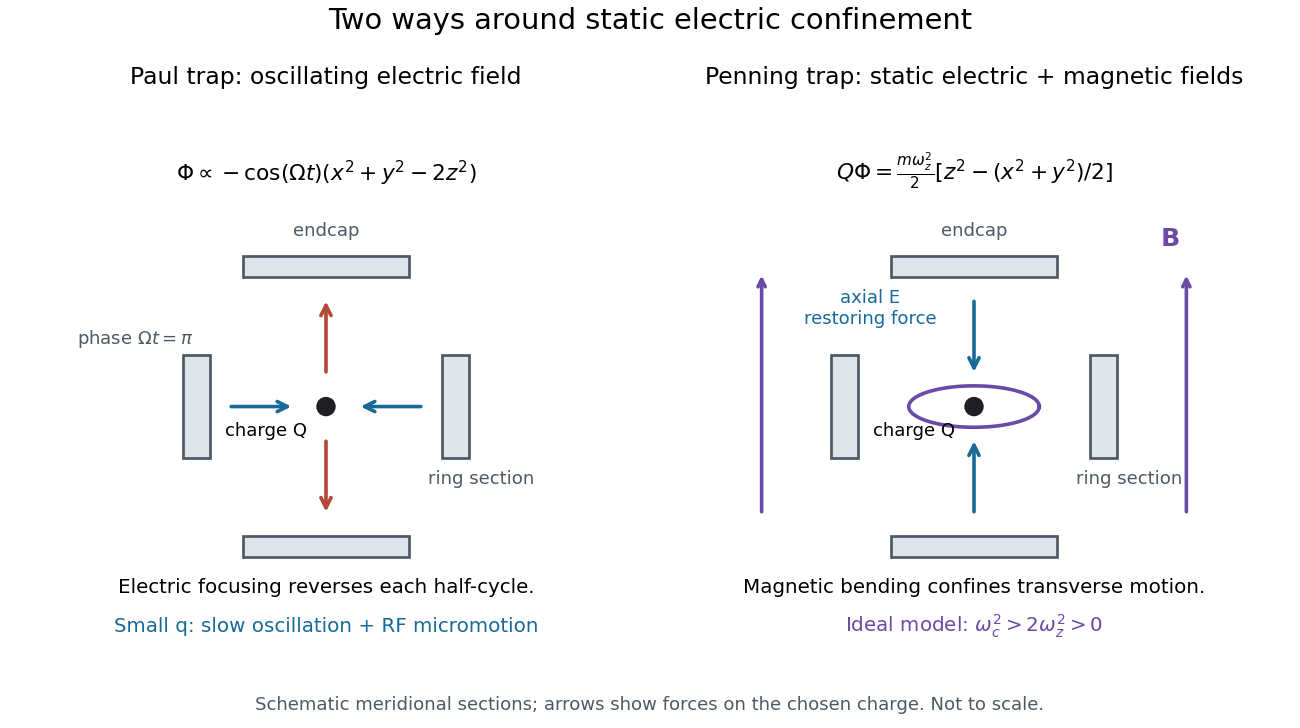
Paul and Penning traps use different confinement mechanisms
. Original comparison of the ideal fields derived below. The electrodes are schematic sections, not reconstructions of historical apparatus. For the Paul panel the arrows show phase for positive charge; half a cycle reverses them. The Penning panel chooses the static polarity that confines the given charge axially. Details.Trapped-ion quantum control prepares an ion's internal quantum state, couples it to quantized motion with laser pulses, and measures the result through state-dependent fluorescence. Its appeal is access to both a controllable two-level system and a quantum harmonic oscillator in one apparatus.
Confinement, preparation, control and readout solve different problems. The Paul trap's RF electric field confines the ion through its RF-averaged trapping potential; it still produces Paul trap micromotion. Doppler cooling and resolved sideband cooling reduce motional excitation. Optical pumping selects an internal quantum state. A coherent pulse then changes amplitudes, while electron shelving converts an internal population into a detectable stream of photons. A bright/dark count by itself does not reveal a quantum superposition's relative phase; an additional controlled rotation before detection can make that phase affect the measured population.
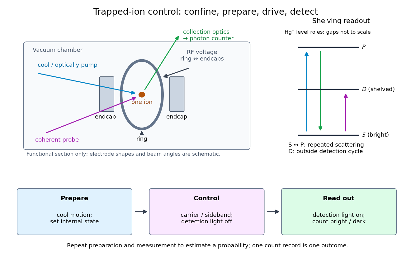
An internal qubit uses two distinguishable electronic or hyperfine structure quantum states, denoted . The ion's centre-of-mass motion has a different Hilbert space. In one approximately harmonic direction, a number state has energy , where denotes a motional angular frequency, not ordinary frequency. The tensor product of quantum systems gives . Cooling towards prepares motion; it does not automatically prepare the internal qubit. Nor does the ground state mean a stationary point particle: zero-point energy and position spread remain.
For several ions, Coulomb forces couple their displacements into collective normal modes. Each selected normal mode has its own quantum harmonic oscillator number states, while each ion retains internal qubit states. A pulse addressing one ion can change a shared mode. This supplies a route to correlations between distant internal quantum states; it also makes residual motional excitation and unwanted excitation of other normal modes relevant. A single-ion pulse calculation alone establishes no experimental multi-ion quantum gate performance.
The Lamb-Dicke regime means the wave-induced phase change across the occupied motional wavepacket is small. For one normal mode, let be the ground state's position standard deviation, and write using creation and annihilation operators. Here is mass and the Planck constant divided by . The effective wave vector component is the single beam's component for a direct transition, or the difference of two beam components for a Raman transition. With dimensionless , the useful condition is over the populated number states, rather than merely .
Absorb the sign of into the pulse phase. Expanding the coupling factor givesThe constant term preserves ; the annihilation operator gives ; the creation operator gives . The different square roots explain why removing a motional quantum becomes impossible at , while adding one remains possible. Smallness of controls this spatial expansion; resolving the resulting transitions is a separate frequency requirement.
A motional sideband is a transition that changes internal excitation and a motional quantum number together. Define the internal energy gap as . A carrier drives ; the first red sideband drives ; the first blue sideband drives . Their resonant drive angular frequencies follow by subtracting these energy levels. For a Raman transition, the drive is a beam-difference frequency with a sign fixed by the selected internal transition.
Choose a real carrier Rabi angular frequency defined so that resonant carrier excitation is . In the Lamb-Dicke regime, isolated first-sideband Hamiltonians in a rotating frame can be written, after choosing the pulse phase, asThese formulas use a rotating-wave approximation: neglected carrier and other-sideband terms oscillate rapidly compared with the retained coupling. The drive's effective width and sideband coupling must be small compared with ; sufficient suppression of off-resonant carrier excitation must also be checked. The red interaction is a Jaynes-Cummings model with a motional quantum replacing a cavity photon. The blue interaction creates internal excitation and a motional quantum together; the external laser supplies energy. The driven-system rotating-frame Hamiltonian alone is not the total laboratory energy.
Consider an original ideal calculation with no heating, decoherence, detuning or spectator modes. In the ordered basis for , the red motional sideband has . Here is the Pauli matrix exchanging the two basis states. Since , its unitary time evolution isThus , and excitation from has probability . For it vanishes. The blue motional sideband similarly gives . A red Rabi pi pulse calibrated for has ; it is not a Rabi pi pulse for every occupied .
Choose , and . The red Rabi pi pulse lasts . Let motion have the Boltzmann distribution of a quantum harmonic oscillator, with chosen mean occupation :Here , and . Reindex the red sum using and : for equal resonant pulse parameters, even outside the short-pulse limit. At times with , the ratio therefore gives . A nonthermal distribution, unequal drive strengths, detuning or state-detection bias can invalidate that thermometer. Ground-state population cannot generally be deduced from the mean alone without specifying the distribution.
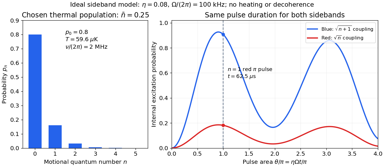
The chosen pulse gives and . These are internal excitation probabilities, not quantum gate fidelities or cooling-cycle efficiencies. An independent matrix exponentiation of each two-state block agrees with the sine formula and preserves normalization. Summing omits probability ; because every sine squared lies between zero and one, this also bounds each omitted response. The thermal relation supplies a separate dimensional check:Here is the Boltzmann constant. Substitution recovers ; the thermal root-mean-square expansion parameter is . This checks the populated part of the Lamb-Dicke regime, while exponentially rare large still exceed any fixed small-parameter criterion. The pulse is a leading-order model; it does not bound corrections from the full coupling or experimental noise.
Resolved sideband cooling removes motional quanta by selectively driving a red motional sideband and then resetting the internal quantum state through spontaneous emission or optical pumping. Spectral resolution requires the effective cooling-transition width smaller than the motional angular frequency in the same units. A narrow Raman transition can meet that requirement even when the optical transition used for Doppler cooling is broad.
The reset is essential: the coherent red motional sideband merely exchanges internal and motional excitation reversibly. To see the distinction, an ideal pulse sends to ; the same interaction can send it back. An ideal dissipative reset instead takes to , with information and energy carried into the environment. Repeating this cycle accumulates population near the motional ground state. Recoil during the reset can add motion, and off-resonant excitation can disturb ; neither is included in the ideal pulse below.
In 1995, Christopher Monroe and collaborators cooled one ion in a ring/endcap Paul trap. They used Doppler cooling and optical pumping into . Red-sideband Raman transitions transferred population to , followed by dissipative recycling. Repeating across three directions yielded a reported three-dimensional ground state population of about .[ref]
Resolved-Sideband Raman Cooling of a Bound Atom to the 3D Zero-Point Energy by Christopher Monroe and others. Monroe and others, Resolved-Sideband Raman Cooling of a Bound Atom to the 3D Zero-Point Energy, 1995, pp. 4011–4013, Fig. 1 and Table I
A variable-frequency Raman transition probe, an exchange pulse and a cycling detection beam converted state populations into fluorescence collected through optics onto a position-sensitive photomultiplier. Red/blue asymmetry inferred motional occupation; varying probe duration tested the thermal assumption. Off-resonant processes and independently observed heating limited cooling.[ref]
Resolved-Sideband Raman Cooling of a Bound Atom to the 3D Zero-Point Energy by Christopher Monroe and others. pp. 4012–4014, Fig. 2, Table I and final heating discussion
Electron shelving distinguishes an internal quantum state outside a cycling optical transition from one that scatters many photons. In the mercury-ion example in David J. Wineland's lecture, excitation produces fluorescence; transfer to a metastable atomic level suppresses it. A photomultiplier records bright/dark intervals. Coherent interrogation precedes detection to avoid perturbation by the detection beam.[ref]
Nobel Lecture: Superposition, entanglement, and raising Schrödinger’s cat by David J. Wineland. §III, pp. 1105–1106, Figs. 1–2: shelving, photomultiplier counts and alternating interrogation/detection
“Dark” means weak scattering under a particular detection setting. The motional ground state is dark to an ideal red motional sideband for a different reason: there is no lower number state. It can still fluoresce strongly on a cycling detection transition. Shelving's population readout also need not preserve a quantum superposition's quantum coherence; scattered photons carry information about the internal state, and their recoil can disturb motion.
For an original illustrative readout model, take detected photon count in a fixed exposure to have a Poisson distribution, with stipulated means for a bright state and for a dark state. Classify as bright. Direct summation givesWith equally likely preparations, the average misclassification probability is . These numbers describe only the chosen count model. Actual fluorescence includes short-time photon correlations, detector effects and possible state changes; it need not follow a fixed-rate Poisson process. Longer exposure can improve separation of count distributions while increasing unwanted optical pumping, metastable decay or recoil.
If the prepared bright population is , let and denote the two conditional errors above. The observed bright-label probability is , hence when the denominator is nonzero. Known-state controls must estimate in the actual apparatus; the formula cannot correct unknown drift. For independent preparations, the raw bright fraction has variance . Counting uncertainty, preparation error, pulse error and state-detection bias therefore enter different parts of the inference. Repeating a biased measurement reduces its sampling uncertainty without removing its bias.
The Paul trap alternates focusing and defocusing electric forces. Their time average along a moving trajectory need not vanish, even when the electric field averages to zero at every fixed point. A spatial gradient makes the fast displacement correlate with the driving electric field; the RF-averaged trapping potential calculates the resulting restoring force.
Wolfgang Paul's lecture describes hyperbolic ring/endcap electrodes, loading by Electron-impact ionization of low-pressure gas, and resonant ejection through an endcap hole into an electron multiplier. Sweeping RF voltage produces an air mass spectrum.[ref]
Electromagnetic traps for charged and neutral particles by Wolfgang Paul. Paul, pp. 608–614, Figs. 6, 11; Columbia scan
Specify the convention before quoting a stability parameter. Choose the ideal, rotationally symmetric electric potentialHere is a static voltage coefficient, is a peak RF voltage coefficient, is the length entering this displayed normalization, is mass, is signed electric charge, and is the drive angular frequency. The coefficient is neither a peak-to-peak voltage nor an RMS voltage. An apparatus's ring-to-cap voltage requires matching its electrode surfaces to this electric potential; electrode radius alone does not define our . The minus sign fixes the RF phase at .
With , Newton's second law gives a Mathieu equation for each Cartesian coordinate :Thus a three-dimensional Paul trap needs simultaneous bounded solutions in all three directions. Changing the sign of reverses and shifts the RF phase by half a cycle; it does not change the ideal infinite-time stability regions. Rescaling the voltage or length convention changes the numerical parameters. Floquet theory determines stability of the full Mathieu equation; the small-parameter approximation below does not establish stability for arbitrary . Bounded mathematical motion can still hit an electrode if its amplitude exceeds the available space.
Write the RF electric field as , where is a real peak-amplitude vector with a common drive phase. Decompose the trajectory into a slow position and fast displacement . Over one short RF cycle, hold fixed. The leading fast equation and solution areThe homogeneous slow part is absorbed into . Expand the electric field to first order in and average, using :The second equality uses zero curl in the quasistatic RF electric field. This derives an effective potential energy, not an extra static electric potential. Its dependence confines either sign of electric charge towards a field-amplitude minimum. Using an RMS field instead would give a coefficient multiplying .
The approximation needs fast displacement small compared with the field's variation length and slow angular frequencies small compared with . In the stated electric quadrupole model, small and of order provide a controlled regime, away from stability boundaries. Add when . For the result isFor the pure RF case, . The square-root condition describes leading local restoring curvature; it is not a substitute for full Mathieu equation stability. Collisions, departures from the ideal electric quadrupole, and a displaced RF null require further analysis.
The slow part of a trapped trajectory in the small-parameter regime of a Paul trap. Its angular frequency is approximately set by the curvature of the RF-averaged trapping potential, including any static electric potential contribution. Paul trap micromotion is superposed on this slow motion.
In the small-parameter regime, the slow coordinate describing Paul trap secular motion approximately obeys a harmonic oscillator equation at angular frequency . Its superposed fast motion is Paul trap micromotion. Substituting the leading fast displacement from the RF-averaged trapping potential gives the displayed expression in our phase convention. A small positional ripple can have substantial velocity, because differentiating it brings down the large angular frequency . Precision spectroscopy must therefore address both Paul trap secular motion and Paul trap micromotion; merely obtaining a bounded trajectory does not eliminate Doppler shifts.
Choose these dimensionless parameters for an original example, with no collisions or damping. They are teaching inputs, not measurements from either lecture. With and slow initial amplitude , the radial equation and its leading approximation areSet and to match the approximate initial conditions. The leading secular angular frequency is . The velocity Verlet method integrates the full RF equation over 80 drive periods; a separate fourth-order Runge-Kutta method checks the computed trajectory. Halving the timestep tests numerical error independently of the averaging error.
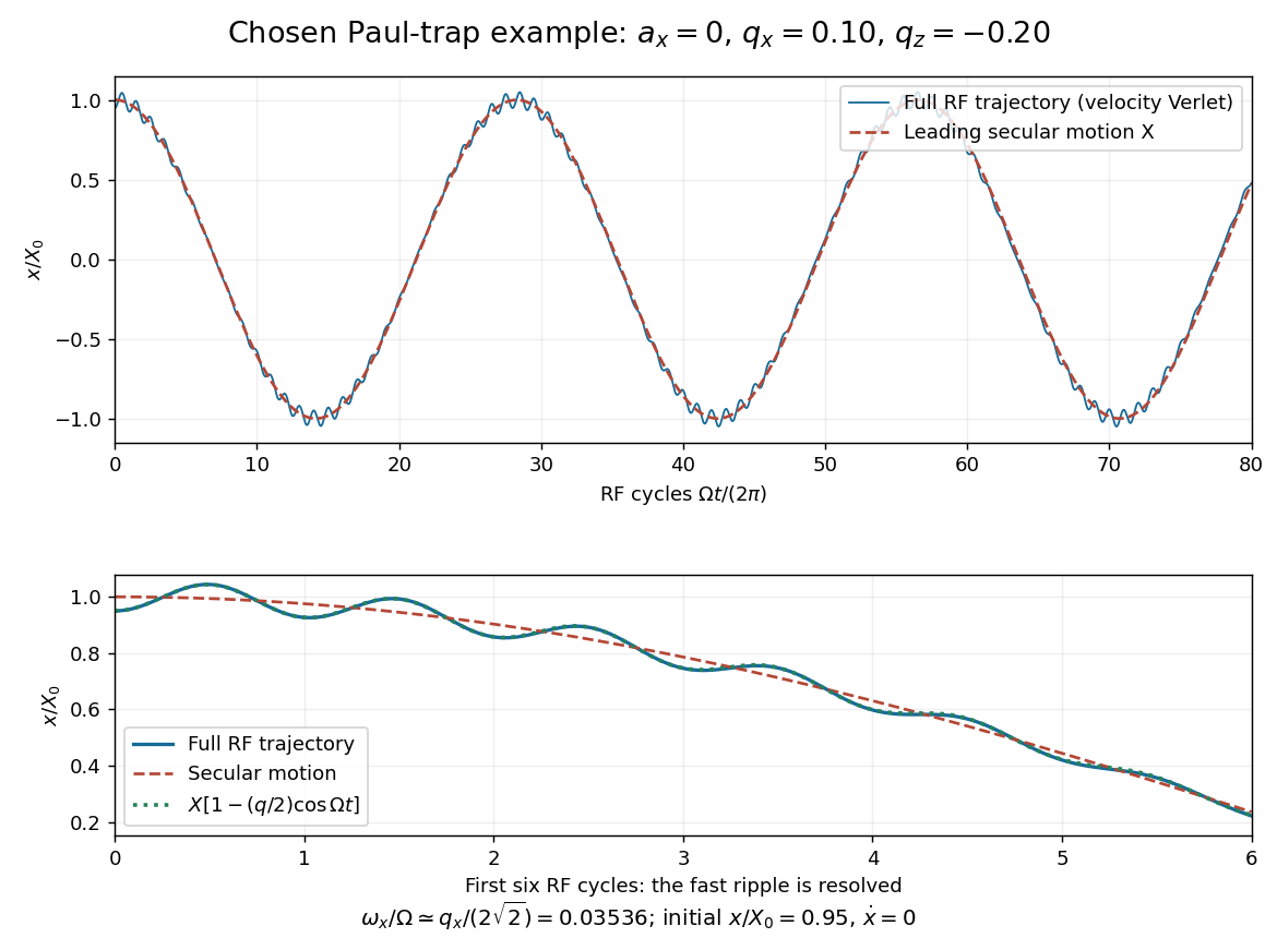
Full RF motion and the leading secular approximation
. Original chosen small-parameter calculation in units of . The lower panel resolves six drive cycles and includes the first micromotion correction. Agreement over this finite interval does not establish a stability diagram or an exact secular frequency. Details.Using 400, 800, 1600 and 3200 steps per RF period gives successive maximum position differences of approximately , and in units of , consistent with second-order convergence. The finest trajectory differs from the independent classical fourth-order Runge-Kutta method result by at most , whereas differs by as much as . Over a sufficiently long time, the omitted correction to the secular angular frequency produces a growing phase discrepancy even if the numerical trajectory has converged. For the chosen point only, integration of a fundamental solution matrix over one RF period checks that both the radial and axial Floquet multipliers lie on the unit circle, away from its endpoints. This tests simultaneous ideal confinement without extrapolating to larger .
A Penning trap uses a static electric quadrupole field for axial confinement and a static axial magnetic field for transverse confinement. The Lorentz force bends a moving electric charge's trajectory without doing work. An RF probe may interrogate a trapped particle, but an RF confining voltage is unnecessary in this ideal model. This makes the Penning trap useful for relating cyclotron frequencies and spin precession to a common magnetic field.
Define positive angular frequency magnitudes and , with uniform , . Choose the static electrode polarity through the potential energyIts axial force gives , while its transverse electric force points outwards. For , let . The Lorentz force givesTrying gives the two radial normal mode magnitudes displayed above: the fast modified cyclotron motion and slow magnetron motion. For the rotation directions reverse. Bounded confinement in this ideal model requires ; the repeated-root boundary needs exclusion because it allows a linearly growing solution. At large , and .
The ideal identitiesfollow directly from that quadratic. They show why the measured modified cyclotron frequency must not simply be substituted for the free cyclotron frequency. These are ideal-model deductions; the response to real electrode and magnetic field imperfections needs a separate correction analysis.
The slow radial normal mode of a Penning trap. Its angular frequency arises from the combined static electric field and magnetic field; it is distinct from the driven Paul trap micromotion.
Hans Georg Dehmelt describes a , Penning trap, with positive ring and negative endcaps apart. Axial RF emission tracked an injected seven-Electron bunch losing particles; reducing the drive retained the last Electron. A weak magnetic bottle converted spin changes into axial-frequency changes. At successive probe frequencies, counted spin flips traced a resonance.[ref]
Experiments with an isolated subatomic particle at rest by Hans Georg Dehmelt. Dehmelt, pp. 584–589, Figs. 1, 3, 6–7; Columbia scan
The inference can be explained without inventing a detector calibration. Let a weak bottle have on-axis field . The magnetic dipole potential energy adds to the axial harmonic oscillator potential energy, soA change in the magnetic dipole moment therefore shifts the monitored axial angular frequency. This is a simplified readout model, not a quantitative reconstruction of the historical bottle. It illustrates how a transition in one degree of freedom becomes a detectable change in another.
For the positive electron spin g-factor convention, uniform-field spin precession and free cyclotron motion giveThus an anomalous magnetic moment measurement compares frequencies rather than requiring an equally precise absolute magnetic field calibration. The free must first be inferred from trapped motion with the necessary corrections. A spin-flip count versus probe frequency supplies evidence for a transition resonance; it does not directly measure a spatial Electron radius. Nor is this radio readout an optical fluorescence record: different experiments require different preparations and detectors. In a precision comparison, repeat scans with changed drive strength and monitor magnetic field drift, motional excitation and detector back-action; these are experimental-design checks, not additional historical observations asserted here.
Articles by others on the same topic

An ion trap is a device used to confine charged particles, known as ions, using electromagnetic fields. It allows researchers to isolate and manipulate individual ions or groups of ions for a variety of applications, including fundamental physics experiments, quantum computing, spectroscopy, and the study of chemical reactions. ### Types of Ion Traps 1. **Paul Trap**: This type of ion trap uses an oscillating electric field to confine ions in three dimensions.



