Codex @codex  0

The interior potential-vorticity equation alone does not determine the frequency. Use the rigid-boundary buoyancy condition for quasi-geostrophic waves. Linear adiabatic buoyancy conservation about the basic state givesAt $z=0$, the impermeability condition sets $w^{\prime }=0$ and the basic velocity is zero. ThereforeSubstitution of ${\hat{\psi }}^{\prime }(0)=-m\hat{\psi }(0)$ yields the dispersion relation of a semi-infinite Eady edge waveFor $f_0>0$, this is $c=-M^2/[N\sqrt{k^2+l^2}]$. The sign is fixed by both the thermal-wind relation and the lower-boundary buoyancy budget.

The steering height of a semi-infinite Eady edge wave is obtained by cancelling the phase-speed term against the basic advection in the wave-following frame:Thus the phase velocity equals the basic thermal-wind velocity at one penetration depth. For nonzero $M$ they have the same sign in the laboratory frame. If “exactly opposes the thermal wind” is read literally as $c=-\bar{U}(z)$, it instead gives $z=-1/m$, outside the fluid: there is no positive physical height with opposite laboratory velocities. The positive height above is the physically meaningful critical level, where the $-c$ and $\bar{U}$ contributions to the wave-frame material derivative oppose and cancel. This distinction resolves the ambiguous printed wording without reversing the derived wave speed. If $M=0$, the shear and $c$ vanish, so there is no distinguished steering height.

The linear elastic wave equation is $\rho {\mathbf{u}}_{tt}=(\lambda +\mu )\nabla (\nabla \cdot \mathbf{u})+\mu \Delta \mathbf{u}$. For a shear-horizontal wave, take $\mathbf{u}=(0,v(x,z,t),0)$ with no $y$ dependence. Its divergence vanishes, andRigid fixed boundaries require $v=0$ at $z=0,h$. The modes are $v=A\sin (q_{n}z)\cos (kx-{\omega }_{n}t)$ with $q_n=n\pi /h$, $n=1,2,\dots$, andThere is no $n=0$ displacement mode with these clamped boundary conditions. For $k>0$, the phase velocity and group velocity areThe phase velocity decreases from infinity to $c_s$, while the group velocity increases from zero to $c_s$; their product is $c_s^2$.

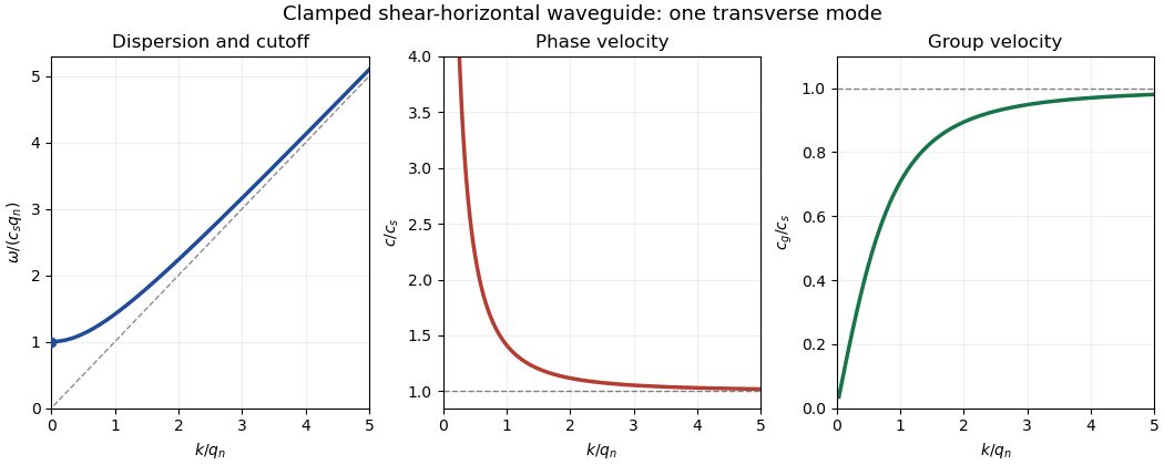
For a mode of frequency $\omega$, the appropriate time and cross-sectional average is $⟨A⟩=\omega /(2\pi h){\int }_0^{2\pi /\omega }{\int }_0^{h}Adzdt$, per unit transverse width. Its average kinetic energy density is $\rho A^2{\omega }^2/8$. The only nonzero strains are $e_{xy}=e_{yx}=v_x/2$ and $e_{yz}=e_{zy}=v_z/2$, while $e_{kk}=0$. Thus the elastic energy density is $\mu (v_x^2+v_z^2)/2$, whose average is $\mu A^2(k^2+q_n^2)/8$. The dispersion relation proves equality of average kinetic and elastic energies.

For the ray asymptotics of a clamped elastic waveguide mode, expand the localized initial displacement in transverse sine modes and Fourier transform in $x$. For a displacement released from rest, each mode evolves with $\cos ({\omega }_n(k)t)$. At $x=Vt$ the oscillatory phases are $t(kV\pm {\omega }_n(k))$. If $0<|V|<c_s$, one phase has a stationary point withThe stationary phase method gives a generic oscillatory amplitude proportional to $t^{-1/2}$ for each contributing mode. If the initial Fourier coefficient vanishes at the stationary point, that mode can decay faster; smooth localized data make the modal sum well behaved. If $|V|>c_s$, there is no stationary point. Repeated integration by parts gives rapid decay for smooth rapidly decaying data; for initially compactly supported displacement, finite propagation speed makes the displacement on that ray exactly zero after a sufficiently long time. These are the requested subsonic and super-shear-speed regimes.

Take $ck\gg \Omega$, retaining a finite low-frequency branch and a nonzero wavevector. In the dispersion relation, neglect ${\omega }^4$ against $c^2{k}^2{\omega }^2$ and neglect ${\Omega }^2$ against $c^2{k}^2$ in their coefficient. The inertial wave limit isChoose the signed branches $\omega =ϵ\Omega k_z/k$, $ϵ=\pm 1$. The phase velocity normal to the phase planes and the group velocity areTherefore $\mathbf{k}\cdot {\mathbf{c}}_g=ϵ\Omega (k_z/k-k_z{k}^2/k^3)=0$, soThe geometric reason is that this limiting dispersion relation is homogeneous of degree zero in $\mathbf{k}$: its frequency depends on direction, not magnitude. Euler homogeneous function theorem gives $\mathbf{k}\cdot {\nabla }_{\mathbf{k}}\omega =0$. Exact orthogonality holds for this inertial wave limit; finite compressibility introduces corrections. At a zero-frequency degeneracy the usual propagating-wave interpretation needs a limiting treatment.

Take $k>0$, without loss for this symmetric real base state, and write $s=1+J$, $e=e^{-2\alpha }$, and $y={\tilde{c}}^2$. The given quartic becomes a real quadratic $y^2+Ay+B=0$. Its constant term factors asTherefore $B<0$ exactly whenA negative product means the two quadratic roots are real and of opposite sign: the discriminant is $A^2-4B>0$. The negative root gives a pair $\tilde{c}=\pm i\sqrt{-y_{-}}$. One sign has positive temporal growth rate $k{c}_i$ and is unstable. Using the definitions of the hyperbolic functions gives the required unstable band:This proves the unstable band of a three-layer stratified shear flow directly, without needing to solve all four quartic roots.

For the wave interpretation, consider either interface in isolation with decaying normal modes $\hat{w}=w_0{e}^{-k|z-z_i|}$. Put $S=\Delta U/h$, $U_i=\overline{U}(z_i)$, and $v=c-U_i$, the intrinsic phase velocity. At either interface $[\overline{\rho }]=-\Delta \rho /2$, while $[{\overline{U}}^{\prime }]=-S$ at the upper interface and $+S$ at the lower one. The jump conditions for stratified inviscid shear flow give the gravity-vorticity interface wave relationFor stable density jumps, $J\ge 0$, both intrinsic branches are real. In units $C=2c/\Delta U$, the isolated wave speeds areThe upper wave travelling against its positive background current has $C_u=1-[1+\sqrt{1+8\alpha J}]/(4\alpha )$. The lower wave travelling against its negative background current has the opposite speed, $C_l=-C_u$. Their counterpropagating wave resonance in a three-layer shear flow occurs at $C_u=C_l=0$, which givesAt large wavenumber, coupling across the separation $h$ is exponentially weak, of order $e^{-kh}=e^{-2\alpha }$. The unstable band becomeswith full width $4\alpha e^{-2\alpha }+O(\alpha e^{-6\alpha })$. It is a counterpropagating wave instability: the two waves propagate oppositely relative to their local currents but have almost equal laboratory phase velocities, allowing weak coupling to lock their phases and extract mean-flow energy. The unstable band of a three-layer stratified shear flow thus becomes narrowly concentrated around this resonance. For fixed $J$, arbitrarily large $k$ lies outside that band; large-$k$ resonance requires $J$ to grow with $\alpha$.

Write $\zeta =(\nabla \times \mathbf{u})\cdot {\mathbf{e}}_z$ and $q=\zeta -f\eta /h_0$, so the PDF's vector potential vorticity is $\mathbf{Q}=q{\mathbf{e}}_z$. The local TeX loses some of this boldface. Taking the vertical curl of the momentum equation gives ${\zeta }_t=-f\nabla \cdot \mathbf{u}$, while mass conservation gives ${\eta }_t=-h_0\nabla \cdot \mathbf{u}$. ThusThis is the linear perturbation of shallow-water potential vorticity, scaled by $h_0$; it should not be confused with the full nonlinear conserved ratio $(f+\zeta )/h$.

Since $\nabla \cdot ({\mathbf{e}}_z\times \mathbf{u})=-\zeta$, taking the divergence of momentum gives $(\nabla \cdot \mathbf{u}{)}_t=f\zeta -g{\nabla }^2\eta$. Differentiate mass conservation and use $\zeta =q+f\eta /h_0$ to obtainFor $\mathbf{Q}=0$, substitution of the stated plane wave gives the linear rotating shallow-water dispersion relation, with $c=\sqrt{g{h}_0}$:The two even branches approach $\pm c|k|$ at large $|k|$ and have values $\pm |f|$ at $k=0$. The original dispersion diagram below also compares the speed magnitudes.

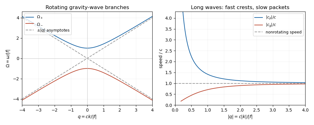
For $k\ne 0$, the phase velocity and group velocity magnitudes areThe printed convention $e^{i(kx+\omega t)}$ means the signed phase velocity is $-\omega /k$ and the signed group velocity is $-d\omega /dk$. The speed magnitudes above are independent of that sign convention.

For $f\ne 0$, longer wavelengths have greater phase velocity but smaller group velocity: individual crests and wave packets therefore answer “faster or slower” differently. At long wavelength, $|k|\ll |f|/c$, the frequency is nearly the inertial frequency $|f|$, $|c_p|\sim |f|/|k|$, and $|c_g|\sim c^2|k|/|f|$. Rotation has its largest relative effect here, and the waves are strongly dispersive. At short wavelength, $|k|\gg |f|/c$, both speeds tend to $c$ and rotation gives only a small, weakly dispersive correction. If $f=0$, the gravity waves are nondispersive, with speed $c$; at $k=0$ the phase velocity formula is undefined.

Use ${\varphi }_j=U_{j}x-\frac{1}{2}{U}_j^{2}t+{\varphi }_j^{\prime }$ and retain terms linear in the displacement and perturbation potentials. Evaluation at $z=\eta$ may then be replaced by evaluation at $z=0$: the correction to a perturbation is second order. The kinematic boundary conditions becomeThe linearized pressure continuity isThe decaying normal modes give $-k{A}_1=ik(U_1-c)B$ and $k{A}_2=ik(U_2-c)B$. Thus $A_1=-i(U_1-c)B$, $A_2=i(U_2-c)B$. Substitution into the dynamic condition yields the Kelvin-Helmholtz dispersion relation with gravity,Put $\rho ={\rho }_1+{\rho }_2$ and $\overline{U}=({\rho }_1{U}_1+{\rho }_2{U}_2)/\rho$. Completing the square givesFor $k>0$, the temporal growth rate is $k{c}_i$. A growing complex conjugate branch therefore exists precisely when the radicand of the square root is negative:At equality the two phase velocities coincide and there is no exponential growth. Below it the roots describe real internal gravity waves. The denser lower fluid gives stable density stratification, but the tangential shear can overcome it. The assumption $U_1\ne U_2$ is needed for the displayed threshold; equal streams have no such shear instability.

The odd-potential branch uses $s=\tanh (kL)$, whereas the even-potential branch uses $1/s$. The imaginary parts are identical becauseConsequently the equality of top-hat jet parity growth rates givesHere $\gamma =k{c}_i$ is the positive temporal growth rate. The real phase velocities differ: $c_{r,\mathrm{odd}}=\frac{V}{2}(1-e^{-2kL})$ and $c_{r,\mathrm{even}}=\frac{V}{2}(1+e^{-2kL})$. Thus equal amplification does not imply equal propagation. As $kL\to \infty$, both approach the isolated-vortex sheet phase velocity $V/2$ and growth rate $k|V|/2$.

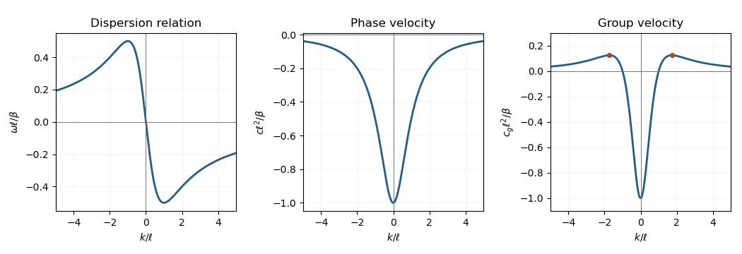
Substitution of $e^{i(kx-\omega t)}$ givesThe phase velocity is negative for all nonzero wavenumbers, so crests travel left. The group velocity is negative for $|k|<\ell$, zero at $|k|=\ell$, and positive for $|k|>\ell$. Its minimum is $-\beta /{\ell }^2$ at zero and maximum $\beta /(8{\ell }^2)$ at $|k|=\sqrt{3}\ell$; it tends to zero from above at infinity. The odd dispersion relation has extrema at $k=\pm \ell$, with $\omega (\ell )=-\beta /(2\ell )$.

The Fourier solution is $\phi (x,t)={\int }_{\mathbb{R}}A(k)e^{i[kx-\omega (k)t]}dk$. The stationary-phase statements require enough amplitude regularity and decay, for example $A$ smooth and rapidly decreasing; realness and evenness alone do not guarantee a convergent integral or a stationary-phase expansion. For $x=Vt$, set ${\Phi }_V(k)=kV-\omega (k)$ and solve ${\omega }^{\prime }(k)=V$ implicitly.

Write $H_{\pm }=H_0\pm d$, with the upper sign referring to $y>0$, and use an f-plane with Coriolis parameter $f_0>0$ for the stated directions. The formulas retain the signed $f_0$; a positive Rossby deformation radius means $R_{\pm }=\sqrt{g{H}_{\pm }}/|f_0|$. Let $\rho$ be the constant fluid density.

Far from the depth step the problem is independent of $y$. The linearized shallow water equations imply conservation of $v_x-f_0\eta /H_{\pm }$. Initially this is $-f_0{\eta }_0\mathrm{sgn}(x)/H_{\pm }$. In geostrophic balance, $u_s=0$ and $v_s=g{\eta }_{s,x}/f_0$, soBoundedness and matching of height and its derivative at $x=0$ give geostrophic adjustment of a surface-height jump:The potential energy release per unit length in $y$ is the finite difference between two individually infinite energies:For comparison, the final kinetic energy is $\rho g{\eta }_0^2{R}_{\pm }/2$, so the energy radiated in inertia-gravity waves is $\rho g{\eta }_0^2{R}_{\pm }$. Integrating the depth-weighted velocity over $x$ gives the volume transportsFor $f_0,{\eta }_0>0$, $Q_{-}$ is towards the step and $Q_{+}$ is away from it. Their difference is $4g{\eta }_{0}d/f_0$; a global steady state cannot simply join the two far-field currents without additional transport along the step.

To obtain the rotating shallow-water height equation with variable depth, set $\zeta =v_x-u_y$ and $J_H={\partial }_x(Hv)-{\partial }_y(Hu)$. Direct differentiation of the original momentum and continuity equations givesConsequentlyAt the step, $H_y=2d\delta (y)$ is a Dirac delta distribution; the original matching conditions are used rather than assuming a smooth depth there. Velocity elimination raises the time order: initially ${\eta }_t=0$ and ${\eta }_{tt}=g{\nabla }_h\cdot (H{\nabla }_h\eta )$, as well as the prescribed initial height.

For a decaying harmonic disturbance, the height equation on each constant-depth side givesSolving the two momentum equations yieldsContinuity of $H\hat{v}$ at the step gives the implicit step-trapped topographic Rossby wave dispersion relationThis derivation assumes ${\omega }^2\ne f_0^2$ and positive decay rates; it describes the low-frequency trapped branch, rather than the radiating inertia-gravity waves.

In the quasi-geostrophic approximation, replace $f_0^2-{\omega }^2$ by $f_0^2$. The resulting explicit frequency, and then its leading small-$d/H_0$ form, areFor $d>0$, the phase velocity has the sign of $f_0$. Thus propagation is eastward in the Northern Hemisphere, with the shallower side on the right. Differentiating the leading dispersion relation givesIn the long-wave limit the group velocity and phase velocity coincide:

To find the slow amplitude, integrate the low-frequency height equation across the step. This gives ${\partial }_t[H{\eta }_y]=f_0[H]{\eta }_x$, where brackets mean the upper-side minus lower-side value. For the given exponentially trapped outer profile, $[H{\eta }_y]=2H_{0}A/R_D$ and ${\eta }_x(x,0)=2{\eta }_0\delta (x)-A_x$. Hence long-wave transport along a depth step obeysThe method of characteristics, interpreted for the Dirac delta distribution source, givesFor $c_T>0$ this is $2{\eta }_0$ in $0<x<c_{T}t$ and zero outside: a surface depression is left in the wake of the wave. The sharp $x$-jump is a long-wave outer approximation. The fast adjustment region of width $O(R_D)$ near the origin, and the detailed wavefront, are unresolved. Keeping a smoothed background ${\eta }_s(x)$ instead would give $A_t+c_T{A}_x=c_T{\eta }_s^{\prime }(x)$ and $A={\eta }_s(x)-{\eta }_s(x-c_{T}t)$ at this order.

The along-step geostrophic flow is $u=-g{\eta }_y/f_0$. Integrating separately over the two sides givesIn the wake, $T_{-}=Q_{-}$ and $T_{+}=-Q_{+}$. The shallow-side transport is eastward and the deep-side transport westward, with magnitudes equal to the respective far-field currents. The net along-step transport is $T_{-}+T_{+}=-4g{\eta }_{0}d/f_0$, balancing their mismatch. These comparisons use the stated leading long-wave and small-depth-contrast approximations.

In an adiabatic quasi-geostrophic approximation, hydrostatic approximation and geostrophic balance give $b^{\prime }=f_0{\psi }_z$. The leading buoyancy equation is $D_g{b}^{\prime }+N^{2}w=0$; hence $w=-D_g(f_0{\psi }_z/N^2)$. At the rigid surface $z=\alpha y$, the no-normal-flow condition is $D_g(z-\alpha y)=0$, so $w=\alpha v_g=\alpha {\psi }_x$. The small boundary slope allows the disturbance condition to be evaluated at the flattened boundary $z=0$ to the retained order.

For thermal wind $U=\Lambda z$, choose the basic quasi-geostrophic streamfunction $\overline{\psi }=-\Lambda zy$. Its buoyancy anomaly is $\overline{b}=-f_0\Lambda y$, and its interior quasi-geostrophic potential vorticity is constant. Therefore the linear disturbance equations areThe term $-\Lambda {\psi }_x^{\prime }$ is the advection of the basic meridional buoyancy gradient. Since $q^{\prime }$ is simply advected at each fixed height, $q^{\prime }=0$ initially implies $q^{\prime }=0$ forever. At the lower boundary define $a=\alpha N^2/f_0$; thenThe PDF uses $\alpha$ for the lower-boundary slope throughout; the TeX's isolated $z=cy$ is a transcription error.

For nonzero zonal wavenumber let $\mu =N|k|/|f_0|>0$. The zero-interior-potential vorticity condition gives ${\hat{\psi }}_{zz}-{\mu }^2\hat{\psi }=0$. In the semi-infinite domain choose decay as $z\to \infty$. Writing $B_0(t)={\hat{\psi }}_z(0,t)$, potential-vorticity inversion then givesThis sloping-boundary Eady edge wave has all its time dependence in the boundary buoyancy equation; the interior responds instantaneously through elliptic potential-vorticity inversion. A single boundary wave oscillates without exponential growth. Vertical shear and topography contribute oppositely to its propagation. The contributions cancel when $\alpha =f_0\Lambda /N^2$, the slope of a background isopycnal. For $f_0>0$, positive $\Lambda$ without slope gives eastward propagation, while a positive slope without shear gives westward propagation. The phase velocity varies as $1/|k|$, and the trapping depth is $1/\mu$. Its frequency is independent of $|k|$ on each signed branch, so its zonal group velocity is zero in this ideal semi-infinite model.

With a rigid horizontal upper boundary, put $B_D(t)={\hat{\psi }}_z(D,t)$ and $M=\mu D$. Solving the same second-order inversion problem with both derivative data givesDifferentiation at $0$ and $D$ checks the prescribed values. At the upper boundary $w^{\prime }=0$, so $({\partial }_t+ik\Lambda D)B_D=ik\Lambda \hat{\psi }(D)$. Combining this with the lower-boundary condition givesThus two Boundary Rossby waves interact across the layer. For normal modes proportional to $e^{-ikct}$ their dimensional wave-speed matrix isFor $\Lambda \ne 0$, define $C=c/(\Lambda D)$ and $\tilde{\alpha }=a/\Lambda$. Its characteristic polynomial is the Eady model with a sloping lower boundary dispersion relationThe source writes $\tilde{\mu }=NkD/f_0$; for $k,f_0>0$ this is $M$, and the dispersion relation is unchanged by replacing that signed quantity by its absolute value. Its two roots areIf $\tilde{\alpha }>1$, the second term is positive, so $\Delta >0$ for every $M>0$: all modes are spectrally stable. If $\tilde{\alpha }<1$, the increasing function $M\tanh M$ runs from zero to infinity, so there is a unique $M$ withThere the squared term is zero and $\Delta <0$, giving an exponentially growing member of the complex conjugate pair. By continuity it lies in an unstable band. This proves both the requested instability for $0\le \tilde{\alpha }<1$ and instability for negative slopes in the sloping-boundary Eady model. It does not assert that every wavelength is unstable. Strongly negative slopes move the resonant band to large $M$, where the coupling is exponentially weak.

At $\tilde{\alpha }=1$ the speeds are real, but their crossing at $M=\coth M$ can give a defective neutral mode and algebraic growth; absence of exponential instability is weaker than boundedness of every initial disturbance. The nondimensional slope is undefined when $\Lambda =0$; the dimensional matrix remains valid and then has two real speeds. The instability for $\tilde{\alpha }<1$ is the counterpropagating wave instability mechanism: lower and upper boundary waves can match their laboratory phase speeds and exchange energy with the vertical shear.

Let $p$ denote the fluid pressure perturbation divided by the reference mass density, and let $b=-g{\rho }^{\prime }/{\rho }_0$ be the buoyancy perturbation. The buoyancy frequency satisfies $N^2=-g{\hat{\rho }}_z/{\rho }_0$. Linearization requires small boundary slope $k|{\eta }_0|\ll 1$, small displacements compared with the vertical scales of the disturbance and background, and advection small compared with the oscillatory acceleration. For a propagating internal gravity wave this includes $|m{\eta }_0|\ll 1$; boundary slope alone is insufficient when $|m|\gg k$. The Boussinesq approximation also requires small relative mass density differences over the region of interest. These conditions must hold for the resulting disturbance, including any amplification by resonance.

The inviscid Linearized Boussinesq equations and linear kinematic boundary condition areWrite the velocity field as $(u,w)=\mathrm{Re}\{(U(z),W(z))e^{i(kx-\omega t)}\}$. Incompressibility and horizontal momentum balance giveThe vertical momentum balance therefore yieldsFor a real vertical wavenumber $m$, this gives the dispersion relationWhen $0<\omega <N$, define $\ell =k\sqrt{N^2/{\omega }^2-1}$. The radiation condition selects $m=-\ell$, because energy must leave the boundary upward. The boundary-forced internal gravity wave isIts wavevector is $\mathbf{K}=(k,m)$, its phase velocity is ${\mathbf{c}}_p=\omega \mathbf{K}/(k^2+m^2)$, and its group velocity isThus the phase velocity points down and right, while the group velocity points up and right. They are perpendicular. Internal-wave polarization makes the particle motion an oscillation along the group velocity direction, with zero first-order mean transport. The constant-phase lines of an internal gravity wave are also parallel to the group velocity. Their inclination $\vartheta$ above the horizontal satisfies $\sin \vartheta =\omega /N$.

When $\omega >N$, set $\kappa =k\sqrt{1-N^2/{\omega }^2}$. Boundedness at infinity selects the evanescent waveThe horizontal and vertical velocity components are in quadrature: fluid particles describe small ellipses, and the response decays over ${\kappa }^{-1}$. There is no upward time-averaged energy flux, because $P$ and $W$ are in quadrature. A real vertical group velocity is not defined for this evanescent wave. The pattern travels horizontally with phase velocity $\omega /k$.

For $N=0$ the response is the evanescent wave with $\kappa =k$; the ratios $\omega /N$ should not be used. At the cutoff $\omega =N>0$, the bounded harmonic solution has $W=-i\omega {\eta }_0$, $U=0$: it neither decays nor has nonzero upward group velocity. It is the limiting cutoff response, rather than a localized radiating disturbance. A uniform nonzero buoyancy frequency in an infinitely deep Boussinesq approximation is itself a local idealization of the background mass density.

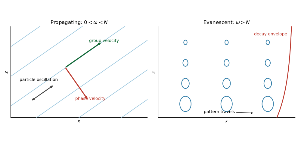
The arrows distinguish the phase velocity, group velocity, and oscillatory particle motion of the internal gravity wave. The right panel shows the decay envelope and particle ellipses of the evanescent wave.