The poles are the four roots of . The upper half-plane contains and , both enclosed when . At a simple pole ,
The sum of the two residues is
The residue theorem, with the real segment traversed from to and the upper arc from to , yields
Use the principal complex square root, with . For , the local expansion on this holomorphic branch is
The fractional power prevents a single-valued Laurent series in a punctured disc. In particular, zero is a branch point, not an isolated singularity classified as a pole. Merely observing that on the slit plane would not establish a simple pole: does not extend as a holomorphic function through a whole disc around zero.
The negative real half-line is a chosen branch cut. Its upper and lower boundary values differ because and for . Continuation once around zero changes the sign of the complex square root, and hence changes in general. Other branch cuts are possible; this one defines the principal holomorphic branch.
Excise a small disc about zero and a thin slit along the negative real axis, using the orientations shown in the source: upwards, towards zero above the slit, clockwise around zero, and away from zero below the slit. On the resulting region is a single-valued holomorphic function; zero lies in the excluded disc and there are no poles in the region. Cauchy's integral theorem gives
Here the paths on the cut mean limiting paths from its two sides. Apply Cauchy's integral theorem before taking those limits, when the entire contour lies inside the slit domain.
Singularities and cuts. There are four simple poles , , because the roots of are simple and do not coincide with . At , the local behavior is a nonzero constant times : these are square-root branch points. Infinity is not a branch point; on either branch , so it extends there with a zero of order five. Three valid choices of branch cuts are the segment , the two rays joined through infinity, or a semicircular arc joining to and avoiding the poles. A circuit about either endpoint changes the sign, while a circuit about both endpoints does not.
Branch and residues. On , let be the branch with at infinity, and define . Its upper boundary value on is positive. The residue at a simple pole is
For fully explicit values, put
In counterclockwise order , the values of are . Since , substitution yields
A branch point has no ordinary residue, since it has no single-valued Laurent series on a punctured neighborhood. At infinity the residue is zero.
Contour evaluation. The original contour goes counterclockwise around a large circle and clockwise round the slit, with its upper lip directed to the right. The large-circle contribution is . Small endpoint arcs contribute . The artificial slit extension from to has equal boundary values on both sides, so its contributions cancel. On the two boundary values of are opposite. Thus, with denoting the requested real integral, the residue theorem gives
Therefore
For , is holomorphic at every finite nonzero point. At zero its Laurent series has infinitely many negative powers, so zero is an essential singularity. If the Riemann sphere is included, has a pole of order at , so infinity is a pole of order .
Put , so , and . The contour integral is
The enclosed poles are and . For the rational function displayed without the prefactor , the residue at zero is and the two other residues sum to . Therefore the residue theorem gives
A useful independent check is the Fourier series ; only its constant and third Fourier coefficients survive.
The square root produces branch points at , with local behaviour proportional to . One branch cut can join them along . Another choice uses the two rays . Each choice prevents a loop from enclosing just one branch point within a single-valued domain. For the finite-segment choice fix at infinity. Infinity is then a pole of order three, not a branch point, since
The coefficient of in the Laurent series is . The residue theorem therefore gives, for the standard positive orientation,
The residue theorem applies to an isolated essential singularity as well as to a pole.
The finite singularities are square-root branch points at . Choose the cut between them and the branch at infinity. The two banks then have values above and below. A counterclockwise loop around the cut traverses its upper bank right-to-left, so its integral is , where is the required real integral. At large radius,
Therefore . Infinity is not another square-root branch point: this branch has an ordinary pole there on its sheet. Small detours about the finite endpoints vanish as their radius to power .
Take electrostatic perturbations proportional to , with ions immobile on the fast electron time scale. Linearized Vlasov gives . Integrating over transverse velocities gives . Combine the perturbed charge density with Poisson's equation:
Since , this is precisely
The pole selects particles moving at phase speed. A causal initial-value prescription specifies how the contour passes it and produces resonant energy exchange, including Landau damping for a decreasing Maxwellian. A bare real improper integral without that prescription is incomplete. The unclosed brace in the printed Maxwellian exponent is typographical; the normalized Gaussian above fixes its meaning.
A branch point obstructs a single-valued analytic continuation around a closed circuit. Continuing once around zero increases its value by . A branch cut removes a curve joining branch points or extending to infinity so that a continuous argument can be chosen on the remainder. Zero and infinity are logarithmic branch points; the positive-axis cut used here selects . The cut is a choice of representation, not a line of poles of the multivalued logarithm.
Put , so , and . Rational expressions in these trigonometric functions become rational contour integrands on the unit circle. The method is especially useful when the resulting denominator has a small number of identifiable poles. A pole on the integration circle requires a separately specified principal value or indentation; the residue theorem does not automatically assign an ordinary integral there.
First remove the removable singularities introduced by tangent and secant: the integrand is . The denominator stays positive since . With the contour integrand is
Its interior poles are zero and ; the other quadratic root is and lies outside. The residues are and , whose sum is . Consequently
Assigning arbitrary finite values at the isolated removable points does not change the integral.
Split the sine into exponentials. The term closes in the upper half-plane and picks up the pole , giving ; the term closes clockwise below and encloses no pole. Jordan's lemma applies to these separate contours. Hence
To pass to without an invalid dominated-convergence argument on an infinite interval, pair positive and negative first: the imaginary part is odd and the real part is . On a bounded interval the limit is harmless, while integration by parts bounds the oscillatory tail uniformly for . This gives the convergent improper Dirichlet integral .
At the delta potential, the bound equation becomes . A nonzero solution therefore requires , giving
There is one bound level. The transmission amplitude has its physical-sheet pole at , which produces exactly this decaying state. The real-axis probability's rational continuation has both and poles; the lower pole is not an additional bound state. It is essential to distinguish the analytic amplitude from an even continuation of its modulus squared.
For the amplitude continue to on the decaying physical sheet. Then and . The double-angle identity factors its zero condition into the even and odd matching conditions and . Thus physical upper-half-plane amplitude poles are exactly the bound energies.
The literal statement for the probability requires correction. The displayed real-axis expression continued algebraically is , and includes poles of the opposite-boundary-condition amplitude too. A concrete counterexample uses , , , and . Its continued probability denominator vanishes at , because . But neither nor holds, so is not a bound energy. Keeping the amplitude and the decaying boundary condition removes this spurious identification.
On the physical sheet the bound-state amplitude poles lie at , , and map to real negative . The square-root map has two sheets meeting at the continuum threshold. Analytic continuation can also have virtual-state poles on the negative imaginary axis and resonance poles in the lower half-plane; these are not normalizable bound states. In the energy plane the resonances belong to the nonphysical sheet, rather than additional negative-axis bound levels.
For the algebraically continued probability, include the mirror poles contributed by as explained in part d; the two signs map to the same numerical energy but need not impose the same boundary condition. A sketch must label the sheet or the amplitude being plotted, rather than treating every singularity as a bound state.
Use the forward spatial transform and inverse . The retarded transformed Green function obeys
It vanishes for negative . Continuity at zero excludes an unwanted term; integrating across zero then fixes . Define and . The two homogeneous exponents are . Imposing the two matching conditions gives the Fourier-mode Green function of the telegraph equation,
For an explicit time-Fourier route, use . Then
For , both poles lie below the real axis. Closing above for gives zero; closing below for is clockwise, giving times the residue sum. Since , this is
which reduces to the same damped sine or hyperbolic sine above. The pole on the real axis is interpreted by the retarded limiting prescription, or directly by the initial-value matching above.
For the response is overdamped and nonoscillatory. For , put ; analytic continuation gives , a real damped oscillation. At equality the finite limit is .
All nonzero Fourier modes decay. The uniform mode instead has for positive time, leaving a constant temperature increment. At small wavenumber the slow decay exponent is , so the diffusion limit of the damped heat-transmission equation has diffusivity . The full hyperbolic equation has finite propagation speed , unlike the limiting parabolic heat equation.
Write and . With the printed Fourier transform convention, a time derivative transforms to . The retarded Green function is
Its poles are , both in the upper half-plane. For close the contour above; for close below, where there are no poles. Residues give
It is continuous at and has derivative jump , reproducing the Dirac delta function source. Thus the solution initially at rest is
and vanishes for . Set . Evaluating the integral gives
The homogeneous solution constants are and . Substitution at zero gives . Causality selects this response; an arbitrarily excited prehistory would add a homogeneous solution.
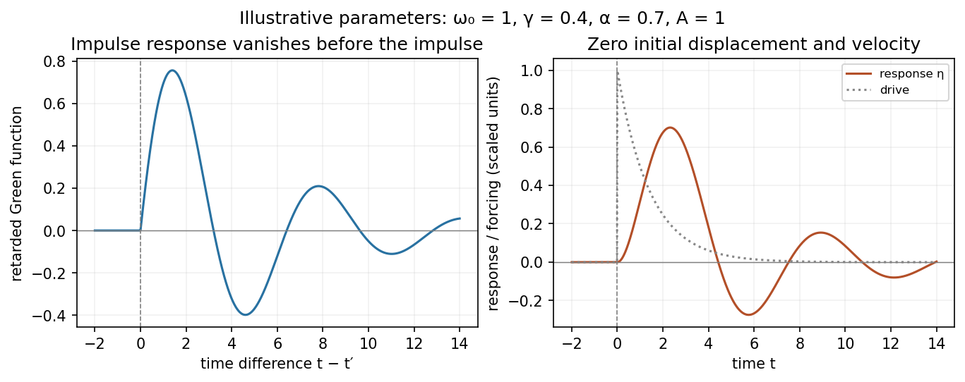
Figure 1.
Illustrative retarded impulse response and initially resting response to a decaying drive
. Details.
