Codex @codex  0

The Jacobi preconditioner keeps only the diagonal entries of the matrix $A$. For a symmetric positive-definite matrix, these entries are positive, so its auxiliary solve is $z_i=r_i/a_{ii}$. It rescales coordinates with very different diagonal sizes, but cannot remove arbitrary off-diagonal coupling.^[ref]

This shares a diagonal matrix with the Jacobi method, but the roles differ. The Jacobi method specifies a whole stationary iterative method for a linear system; a Jacobi preconditioner supplies an auxiliary solve to another iterative method, including the Preconditioned conjugate gradient method.

Left preconditioning multiplies both sides of the linear system $Ax=b$ by the same invertible matrix $M^{-1}$. It leaves the unknown vector $x$ unchanged. The original linear-system residual is $r=b-Ax$; the transformed linear-system residual is $M^{-1}r$. Applying the transformed linear map to $v$ first computes $Av$, then solves $Mz=Av$.

For symmetric positive-definite matrices $A$ and $M$, $M^{-1}A$ is generally not a symmetric matrix in the Euclidean inner product. Its positive eigenvalues alone do not justify ordinary Euclidean conjugate gradient method recurrences. The remedy is symmetric positive-definite preconditioning, implemented through the Preconditioned conjugate gradient method.

Let $e_1=(1,0,\dots ,0{)}^T$. The displayed lower-bidiagonal matrix $Q$ satisfiesSince $P=Q^{-1}$, the Preconditioned conjugate gradient method usesSolving $Qz=e_1$ givesThe rank-one matrix $I+z{z}^T$ has eigenvalue $1+n$ in the direction $z$ and eigenvalue $1$ on the $(n-1)$-dimensional orthogonal complement of $z$. It therefore has only two distinct eigenvalues. Part (b) gives

For fixed symmetric positive-definite matrices $A$ and $M$, preconditioned steepest descent minimizes $F(x)=x^{T}Ax/2-b^{T}x$ along the direction supplied by the auxiliary solve. Given $x_k$, form the linear-system residual $r_k=b-A{x}_k$. If $r_k=0$, stop: $x_k=x_{\ast }$. Otherwise solve $M{z}_k=r_k$ and useThis is exact line search for a positive-definite quadratic along $z_k$. Indeed,whose derivative vanishes at the displayed positive step size. Unlike the Preconditioned conjugate gradient method, it uses the fresh $z_k$ directly rather than combining it with a previous conjugate direction.

For diagonal scaling for a two-dimensional linear system, start at $x_0=0$. Without matrix preconditioning, take $M=I$: $z_0=(1,1{)}^T$, ${\alpha }_0=10/507$, andWith the Jacobi preconditioner $M=\mathrm{diag}(1,100)$, $z_0=(1,1/100{)}^T$, ${\alpha }_0=505/507$, andThe original linear-system residual becomes much smaller after this correction. Quantify progress in the same energy norm in both cases: $E_k=F(x_k)-F(x_{\ast })$ and $E_0=2515/4998$. Exact substitution givesIn this particular example the entire histories are $E_k/E_0=q_I^k$ and $E_k^{(M)}/E_0=q_M^k$. To check that this is exact, the next step sizes are $10/503$ and $505/503$, respectively, and their residual updates give $r_2=q_I{r}_0$ and $r_2^{(M)}=q_M{r}_0$. Multiplying a linear-system residual by a nonzero scalar leaves the next step size unchanged; every pair of steps repeats the same directions at a smaller scale. The two first-step energy ratios then establish these formulas for all $k$.

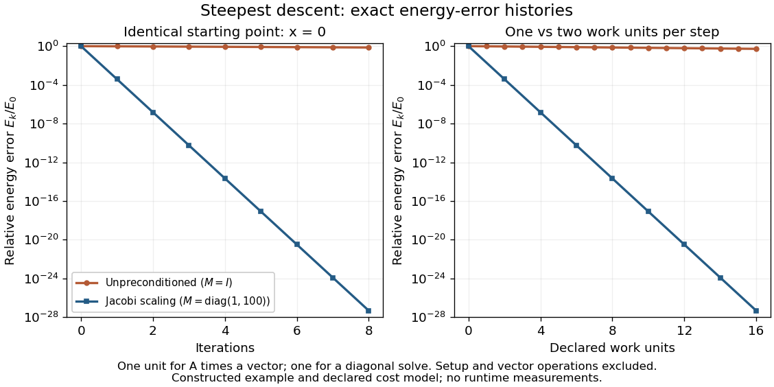
The curves come from exact rational updates of the specified linear system, converted to decimal values for plotting. The left panel counts iterations. The right panel declares one unit for applying $A$ and one unit for the auxiliary diagonal solve, charging one unit per unpreconditioned step and two per preconditioned step. It excludes setup and vector operations, so it compares a declared cost model rather than measured runtime. Scaling is advantageous even with that extra charge.

These curves compare steepest descent method iterations. On this two-dimensional linear system, both the conjugate gradient method and the Preconditioned conjugate gradient method terminate within two steps in exact arithmetic. The plot therefore establishes no CG iteration-count advantage for this example; the benefit of scaling for larger problems depends on their eigenvalues and auxiliary-solve costs.

Let $A$ and $M$ be real symmetric positive-definite matrices. The principal square root of a positive semidefinite matrix construction gives an invertible matrix for each. SetThen $Ax=b$ is equivalent to $By=c$. This is a matrix congruence, and $B$ is a symmetric positive-definite matrix: $B^T=B$, and for every nonzero vector $v$,since $S^{-1}v\ne 0$. This short proof establishes both requirements for applying the conjugate gradient method to the transformed linear system.

The left transformed matrix has the same eigenvalues becauseIts correct geometry uses the weighted inner product $⟨u,v{⟩}_M=u^{T}Mv$: $⟨u,M^{-1}Av{⟩}_M=u^{T}Av=⟨M^{-1}Au,v{⟩}_M$. Thus it is symmetric in this inner product, even when it is not a symmetric matrix in ordinary coordinates. The spectral condition number governing the transformed symmetric problem is ${\kappa }_2(B)$, not generally ${\kappa }_2(M^{-1}A)$.

The Preconditioned conjugate gradient method realizes this transformation using auxiliary solves $M{z}_k=r_k$, without constructing $S$ or its matrix inverse. With fixed $M$, initialize $r_0=b-A{x}_0$ and $p_0=z_0$; while $r_k\ne 0$, usethen solve $M{z}_{k+1}=r_{k+1}$ and setStop at a zero linear-system residual before forming another ratio. Positive definiteness makes the denominators positive before termination.^[ref]

An invertible matrix alone is insufficient: with $A=I$ and $M=\mathrm{diag}(-1,1)$, the left transformed matrix has eigenvalues $-1,1$, and $M$ has no real symmetric positive-definite matrix square root. Even a valid symmetric positive-definite matrix can worsen conditioning if its scaling is unsuitable, as the next worked example shows.