Codex @codex  0

The command centres the log measurements and performs principal component analysis of their covariance matrix. With cor=F, it does not first standardize the variables to variance one. For a unit principal component loading vector $q$, the score $q^T(z_i-\bar{z})$ has sample variance $q^T\hat{\Sigma }q$. By the spectral theorem for real symmetric matrices, expand $q$ in an orthonormal eigenbasis; that variance is a weighted average of the eigenvalues. Its maximum is the largest eigenvalue, reached at the corresponding eigenvector. Repeating subject to orthogonality to previous directions gives the other principal components.

The software uses the divisor-$31$ sample covariance matrix for its component standard deviations, whereas var used divisor $30$. Diagonalizing the displayed matrix gives approximatelyTaking square roots of the latter gives $(0.5671603,0.07312405,0.03064834)$, agreeing with the output to the rounding of the displayed sample covariance matrix. The normalization changes these numerical standard deviations but leaves the eigenvectors and proportions of explained variance of a principal component unchanged.

The first principal component explains about $98.08\%$ of the total log-variable variance, the second another $1.63\%$, and the last about $0.286\%$. Keeping two preserves about $99.714\%$. An original scree plot displays the sharp drop after the first component:

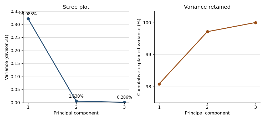
Consequently the centered cloud is very elongated along one direction: a one-dimensional approximation represents almost all of its squared variation. From the displayed covariance matrix, a unit first eigenvector, with its arbitrary sign chosen positive, is approximatelyIts principal component score is therefore $0.3980(\log G_i-\overline{\log G})+0.09514(\log H_i-\overline{\log H})+0.9124(\log V_i-\overline{\log V})$. All coefficients have the same sign, so this direction describes overall tree size, with log volume dominating the unstandardized variation. The summary alone supplies proportions, not the loading directions; the displayed sample covariance matrix supplies the latter. This is a geometric approximation, not evidence of an exact deterministic relation or independent original variables.

One further use is principal component analysis on a correlation matrix, obtained with cor=T, which equalizes marginal variances and answers a different scaling-sensitive question. Another is principal component regression: fit a response to selected principal component scores rather than highly correlated original predictors, choosing the number using prediction assessment. The fitted transformation also projects new measurements into the same low-dimensional coordinates, provided the training centering and scaling are retained.

The new score columns are orthogonal, since $Z^{T}Z=V^T{X}^{T}XV$ is diagonal. This decouples the slope normal equations; with positive eigenvalues and the stated error covariance, the two estimated score coefficients are uncorrelated. It also makes variance explained and possible dimension reduction explicit.

The trade-off is interpretation: each principal component is a mixture of the original variables, so its regression coefficient is less directly connected to changing one original input. Keeping both components is an invertible reparameterization and gives exactly the same fitted values and residual sum of squares. It does not repair a zero eigenvalue or remove instability associated with a very small one. Dropping a low-variance component may improve numerical stability and reduce estimator variance, but changes the model and can discard predictive information, since principal component analysis uses predictor variance rather than the response. This is the distinction between a full rotation and principal component regression with truncation.

The polymerase chain reaction amplifies a selected DNA region using repeated copying steps. Amplified material can be examined by DNA sequencing; appropriate template controls help distinguish a new rearrangement from material already present in the starting preparation.

The essential trick is to choose two PCR primers on opposite DNA strands with their extendible $3^{\prime }$ ends facing into the same interval. A DNA polymerase extends each PCR primer $5^{\prime }\to 3^{\prime }$; the resulting DNA can itself become a template. The amplicon is therefore selected by two opposed PCR primers, rather than by the DNA polymerase recognizing a named gene. This makes PCR amplification useful for inspecting one interval within a much larger genome. Here PCR means polymerase chain reaction; the statistical abbreviation PCR means principal component regression.^[ref]

For a deliberately tiny nucleotide sequence example, display the upper strand as $5^{\prime }\text{-}\mathrm{ACGT}\text{-}\mathrm{GGAATT}\text{-}\mathrm{CAGC}\text{-}{3}^{\prime }$. The left PCR primer is $5^{\prime }\text{-}\mathrm{ACGT}\text{-}{3}^{\prime }$ and binds the lower strand. The right PCR primer, written in its own $5^{\prime }$-to-$3^{\prime }$ direction, is $5^{\prime }\text{-}\mathrm{GCTG}\text{-}{3}^{\prime }$: the reverse complement of CAGC. It binds the upper strand and extends leftward in the drawing. With flanks outside this interval, the bounded amplicon contains $4+6+4=14$ base pairs, including both PCR primer sequences. These four-nucleotide PCR primers illustrate direction and counting only; they are not a proposed experimental design.

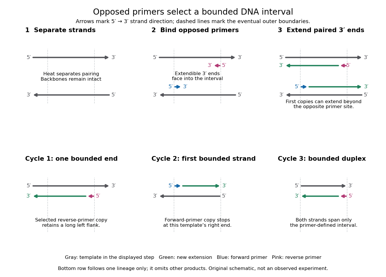
A useful way to understand the polymerase chain reaction is to separate recognition from construction. Base pairing positions a PCR primer; a DNA polymerase then joins new nucleotides onto that existing strand. The PCR primer becomes part of the copied DNA, rather than merely marking a place for an independent strand to start. A PCR thermal cycle repeatedly exposes templates, positions starting ends and permits construction. This makes DNA copying possible outside biological cells, with the chosen PCR primers specifying which interval is repeatedly accessible.