Codex @codex  0

Integrate the probability density function over the specified interval:The endpoint inclusions make no difference for this continuous distribution.

Integrating the first probability density function gives the cumulative distribution functionIts graph is a straight ramp from $(0,0)$ to $(T_1,1)$, followed by a horizontal plateau.

The graph of the positive-delay probability density function is a horizontal segment at height $1/R$ from $s=0$ to $r$, followed by zero from $r$ to $R$. Values at individual endpoints do not affect probabilities. The separate atom $1-r/R$ at zero is not a finite-height part of this density graph.

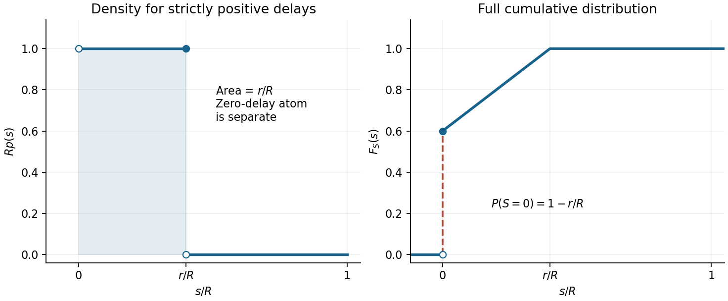
The companion cumulative distribution function in the figure is $F_S(s)=0$ for $s<0$, $F_S(s)=1-r/R+s/R$ for $0\le s<r$, and $F_S(s)=1$ for $s\ge r$. Its jump at zero displays the discrete part without confusing density height with probability mass.

For $s>0$, integrate the probability density function to obtain the cumulative distribution functionIf $\mu >0$, the requested probability is $F_X(\mu )-F_X(0)$. Since the hyperbolic tangent is odd, this givesThe second case matters because the question places no sign restriction on $\mu$: the event is empty when its upper endpoint is nonpositive. Using an oriented integral from $0$ to a negative $\mu$ would give a negative number, not a probability.

A probability density function must be nonnegative. The printed condition $s\ne 0$ is therefore too weak: for $s<0$ the given prefactor makes the function negative everywhere. The location-scale form of the logistic distribution requires $s>0$, which is assumed in the remaining parts.

Set $t=(x-\mu )/(2s)$, so $dx=2sdt$. The normalization of a probability distribution follows from the antiderivative of the squared hyperbolic secant:For completeness, the same expression with $s<0$ integrates to $-1$, since the transformed limits reverse. If a signed scale were desired, replacing its prefactor by $1/(4|s|)$ would give a valid density, but that is a correction to the printed formula.

The angular interval has width $\pi$, so its continuous uniform distribution has probability density functionIntegrating this probability density function gives the cumulative distribution functionValues of the probability density function at the two individual endpoints may be assigned arbitrarily without changing any probability.

Differentiate the cumulative distribution function using the chain rule:This is a Cauchy distribution with location zero and scale $x_0$. The probability density function is nonnegative and integrates to $F(\infty )-F(-\infty )=1$.

The new angular interval has width $\pi /2$, so its probability density function is $2/\pi$ there. Its endpoints stay away from the poles of the tangent function, making $Y$ bounded and its expected value finite. Integrate over the continuous uniform distribution of angles:The two cosines are $\sqrt{3}/2$ and $1/2$. HenceIt has units of length and is positive because the permitted positive angles extend farther than the negative ones.

Normalization of the probability density function requires $1=\alpha {\int }_0^{\pi }\sin xdx=2\alpha$. Thus

The expected value follows by integration by parts:The same result follows from symmetry of the probability density function about $\pi /2$.

A probability density function must have total integral one. The numerator is an even function, soThis is positive, ensuring nonnegativity of the probability density function.

Put $N=6-2e^{-2}$. The function graph is symmetric about the vertical axis, zero outside $[-2,2]$, and has its unique maximum at $x=0$ with height $2/N$. On $0<x<2$, it decreases as $(1+e^{-x})/N$; the negative side is its reflection. The one-sided interior endpoint values are $(1+e^{-2})/N$, so the probability density function jumps to zero at both ends of its support. It also has a corner at its central maximum because of the absolute value in the exponent.

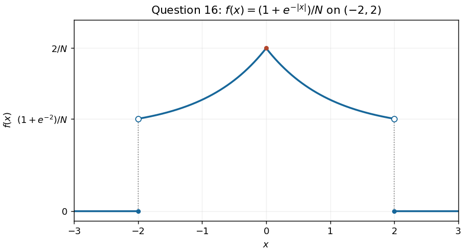
Values assigned exactly at $x=\pm 2$ do not affect any probability.

Since the probability density function is an even function, $xf(x)$ is an odd function. Its integral over the symmetric support vanishes, so

Let $F$ be the cumulative distribution function of $X$. Normalisation of the proposed probability density function requires $M={\int }_{-2}^{2}F(y)dy$. The integrated cumulative distribution function on a bounded interval identity givesFor a direct symmetry proof, the continuous symmetric probability distribution satisfies $F(-y)=1-F(y)$. HenceIn particular $g(y)=F(y)/2$ is nonnegative and has total integral one over its stated support.

The probability density function is the derivative of the cumulative distribution function:It is nonnegative and has integral $F(1)-F(0)=1$. This is a beta distribution with parameters $3$ and $2$.

The probability density function is zero outside $[0,1]$. Inside that interval, it rises from $(0,0)$, reaches its only interior maximum at $x=2/3$, and falls to $(1,0)$. The derivative ispositive for $0<x<2/3$ and negative for $2/3<x<1$. Its maximum height is $f(2/3)=16/9$. The second panel of the figure in part (b) shows the function graph on the requested full range, with this mode marked.

The interior stationary point of the probability density function solves $12x(2-3x)=0$ with $0<x<1$, giving $x=2/3$. The sign change of $f^{\prime }$ established in part (d), together with zero endpoint values, makes this the global maximum. Thus

The graph is a rectangle of height one over $[0,1)$, with zero height elsewhere. Its unit area is the required normalization of the probability density function.

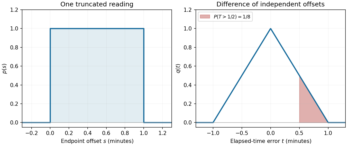
A displayed minute contains one minute of possible start times, so the specified uniform distribution has probability density functionEndpoint choices for a probability density function do not affect any probabilities.

The probability density function graph joins $(-1,0)$ to $(0,1)$ to $(1,0)$ and is zero elsewhere, as shown in the right panel of the timing figure. Its area isThus the probability distribution is normalized.